Lecture 1: Data, visuals and descriptives
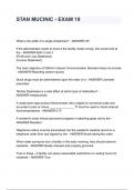
The data matrix or data frame:
Data are put into a Data Matrix or Data Frame (Excel sheet)
- Columns: variables
- Rows: subjects/cases
- Cells: observations of a variable for that specific subject/case
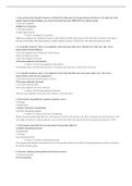
Data types and example:
Determining the measurement level:
Missing data:
Missing data can be dealt with in various ways in
statistical analysis
- Delete missing cases: easy, but loses information
- Impute (cleverly guess) missing cases: for
instance,
o by filling out the mean income if income is
missing
o by filling out the most frequent video
category (if category is missing). This
retains more observations / cases, but
hinges on the correctness of the
imputation assumptions
,Population vs sample:
The population is the collection of all possible data points: typically, we do *not* have it! (e.g.,
the population of ALL 1st year VU business students)
A sample is a subset of data taken from the population. (e.g., the students present today in
this session are a sample of all VU 1st year business students)
- We use this sample to infer something about the population:
o e.g., is there sufficient support for increasing expat subsidies under low-
income residents
o A sample always has an aspect of randomness to it: it could have been a
different sample
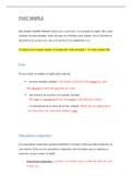
Categorical data:
#occurrences
-Summary measures for categorical data: Proportion: 𝑝 = 𝑛
-Sample proportion = p, population proportion = , population size = N
-Skewness is a measure of asymmetry
-Kurtosis is a measure of tail flatness/fatness → if kurtosis is large, more outliers/huge
outcomes compared to normal cases
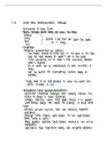
Numerical variables:
∑𝑛 ̅)
𝑖=1(𝑥𝑖 −𝑥̅ )(𝑦𝑖 −𝑦
Sample covariance: 𝑆𝑋𝑌 = 𝑛−1
𝑺
Sample (Pearson) correlation: 𝑺 𝑿𝒀
𝑺 𝑿 𝒀
Correlation is a standardized (scale free) analogue of the covariance: both should
have the same sign.
, Lecture 2: Probability
Event: A is an event (A’ denotes not event A)
Examples: event A can be “heads” in a coin toss (and A’ is then “tails”), or A can be throwing
4 with a fair dice, or having a goal outcome (149,0)
- An event must be inside the sample space, otherwise it cannot occur (it will have
probability zero; in a coin toss throwing “telephone” is impossible)
Probability: P(A) the probability of event A
Notation:
-𝑃 (𝐴 ∪ 𝐵) means probability of either A or B or both A and B happening
-𝑃 (𝐴 ∩ 𝐵) means probability of both A and B happening jointly
-Disjoint: events A and B are disjoint if they cannot happen at the same
time (i.e., probability of A and B together is zero, or 𝑃 𝐴 ∩ 𝐵 = 0)
𝑃(𝐴) 1−𝑃(𝐴)
-Odds for 𝐴: 1−𝑃(𝐴)
; odds against 𝐴: 𝑃(𝐴)
• General law of addition: 𝑃 (𝐴 ∪ 𝐵) = 𝑃 (𝐴) + 𝑃 (𝐵) − 𝑃 (𝐴 ∩ 𝐵)
• Conditional probability: 𝑃 (𝐴 |𝐵) = 𝑃(𝐴 ∩ 𝐵)/𝑃 (𝐵)
• General law of multiplication: 𝑃 (𝐴 ∩ 𝐵) = 𝑃 (𝐴|𝐵) 𝑃 (𝐵) = 𝑃 (𝐵|𝐴) 𝑃(𝐴)
Types of probability:
-Classical: P (event) =
number of elementary outcomes in event
number of possible elementary outcomes
-Empirical: P (event) =
number of elementary outcomes in event
number of observations
Important properties of a probability function P(A)
- For every event A in the sample space: 0 P(A)1
- For entire sample space S, we have P(S) = 1: the probability of obtaining some
outcome out of the set of all possible outcomes is 1
- For disjoint events A and B, we have we have 𝑃 (𝐴 ∪ 𝐵) = 𝑃 (𝐴) + 𝑃 (𝐵)
- However, if events are not disjoint, then 𝑃 (𝐴 ∪ 𝐵) = 𝑃 (𝐴) + 𝑃 (𝐵) - 𝑃 (𝐴 ∩ 𝐵)
The complement of an event 𝐴 is denoted by 𝐴% and consists of everything in the sample
space 𝑆 except event 𝐴 → Since 𝐴 and 𝐴% have no overlap and together comprise the entire
sample space 𝑆, 𝑃 (𝐴) + 𝑃 (𝐴’) = 1 or 𝑷 (𝑨’) = 𝟏 − 𝑷(𝑨)
-The empty set denoted as ∅ contains no elements: 𝑃 ∅ = 0.
𝐴∪B
-The union of two events consists of all elementary outcomes in the
sample space that are contained either in event 𝐴 or in event 𝐵 or in
both
- denoted by 𝐴 ∪ B
- pronounced as “𝐴 or 𝐵” (“or” meaning here “and/or”)
The data matrix or data frame:
Data are put into a Data Matrix or Data Frame (Excel sheet)
- Columns: variables
- Rows: subjects/cases
- Cells: observations of a variable for that specific subject/case
Data types and example:
Determining the measurement level:
Missing data:
Missing data can be dealt with in various ways in
statistical analysis
- Delete missing cases: easy, but loses information
- Impute (cleverly guess) missing cases: for
instance,
o by filling out the mean income if income is
missing
o by filling out the most frequent video
category (if category is missing). This
retains more observations / cases, but
hinges on the correctness of the
imputation assumptions
,Population vs sample:
The population is the collection of all possible data points: typically, we do *not* have it! (e.g.,
the population of ALL 1st year VU business students)
A sample is a subset of data taken from the population. (e.g., the students present today in
this session are a sample of all VU 1st year business students)
- We use this sample to infer something about the population:
o e.g., is there sufficient support for increasing expat subsidies under low-
income residents
o A sample always has an aspect of randomness to it: it could have been a
different sample
Categorical data:
#occurrences
-Summary measures for categorical data: Proportion: 𝑝 = 𝑛
-Sample proportion = p, population proportion = , population size = N
-Skewness is a measure of asymmetry
-Kurtosis is a measure of tail flatness/fatness → if kurtosis is large, more outliers/huge
outcomes compared to normal cases
Numerical variables:
∑𝑛 ̅)
𝑖=1(𝑥𝑖 −𝑥̅ )(𝑦𝑖 −𝑦
Sample covariance: 𝑆𝑋𝑌 = 𝑛−1
𝑺
Sample (Pearson) correlation: 𝑺 𝑿𝒀
𝑺 𝑿 𝒀
Correlation is a standardized (scale free) analogue of the covariance: both should
have the same sign.
, Lecture 2: Probability
Event: A is an event (A’ denotes not event A)
Examples: event A can be “heads” in a coin toss (and A’ is then “tails”), or A can be throwing
4 with a fair dice, or having a goal outcome (149,0)
- An event must be inside the sample space, otherwise it cannot occur (it will have
probability zero; in a coin toss throwing “telephone” is impossible)
Probability: P(A) the probability of event A
Notation:
-𝑃 (𝐴 ∪ 𝐵) means probability of either A or B or both A and B happening
-𝑃 (𝐴 ∩ 𝐵) means probability of both A and B happening jointly
-Disjoint: events A and B are disjoint if they cannot happen at the same
time (i.e., probability of A and B together is zero, or 𝑃 𝐴 ∩ 𝐵 = 0)
𝑃(𝐴) 1−𝑃(𝐴)
-Odds for 𝐴: 1−𝑃(𝐴)
; odds against 𝐴: 𝑃(𝐴)
• General law of addition: 𝑃 (𝐴 ∪ 𝐵) = 𝑃 (𝐴) + 𝑃 (𝐵) − 𝑃 (𝐴 ∩ 𝐵)
• Conditional probability: 𝑃 (𝐴 |𝐵) = 𝑃(𝐴 ∩ 𝐵)/𝑃 (𝐵)
• General law of multiplication: 𝑃 (𝐴 ∩ 𝐵) = 𝑃 (𝐴|𝐵) 𝑃 (𝐵) = 𝑃 (𝐵|𝐴) 𝑃(𝐴)
Types of probability:
-Classical: P (event) =
number of elementary outcomes in event
number of possible elementary outcomes
-Empirical: P (event) =
number of elementary outcomes in event
number of observations
Important properties of a probability function P(A)
- For every event A in the sample space: 0 P(A)1
- For entire sample space S, we have P(S) = 1: the probability of obtaining some
outcome out of the set of all possible outcomes is 1
- For disjoint events A and B, we have we have 𝑃 (𝐴 ∪ 𝐵) = 𝑃 (𝐴) + 𝑃 (𝐵)
- However, if events are not disjoint, then 𝑃 (𝐴 ∪ 𝐵) = 𝑃 (𝐴) + 𝑃 (𝐵) - 𝑃 (𝐴 ∩ 𝐵)
The complement of an event 𝐴 is denoted by 𝐴% and consists of everything in the sample
space 𝑆 except event 𝐴 → Since 𝐴 and 𝐴% have no overlap and together comprise the entire
sample space 𝑆, 𝑃 (𝐴) + 𝑃 (𝐴’) = 1 or 𝑷 (𝑨’) = 𝟏 − 𝑷(𝑨)
-The empty set denoted as ∅ contains no elements: 𝑃 ∅ = 0.
𝐴∪B
-The union of two events consists of all elementary outcomes in the
sample space that are contained either in event 𝐴 or in event 𝐵 or in
both
- denoted by 𝐴 ∪ B
- pronounced as “𝐴 or 𝐵” (“or” meaning here “and/or”)