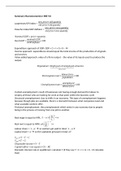
new price∗old quantity
Laspereyes/CPI index =
old price∗old quantity
new price∗new quantity
Paasche index/GDP deflator =
old price∗new quantity
Nominal GDP= price∗quantity
nominal GDP
Real GDP= ∗100
GDP deflator
Expenditure approach of GDP: GDP = C + I + G + X – M
Income approach: expenditures should equal the total income of the production of all goods
and services
Value-added approach: value of a firms output – the value of its inputs used to produce the
output.
Population=Employed
⏟ +Unemployed + Inactive
Labour force
labour force
Participation rate= ∗100
population
unemployed
Unemployment rate= ∗100
labour force
Cyclical unemployment: result of businesses not having enough demand for labour to
employ all those who are looking for work at that point within the business cycle
Structural unemployment: due to shifts in an economy. This type of unemployment happens
because though jobs are available, there's a mismatch between what companies need and
what available workers offer.
Frictional unemployment: the unemployment which exists in any economy due to people
being in the process of moving from one job to another.
K α
Real wage is equal to MPL: ( 1−α ) A ( )
L
=w
L 1−α
Real rent is equal to MPK: αA
K ( ) =r
Labour share = ( 1−α ) so workers get paid in total: ( 1−α ) Y
Capital share = α so the capitalists get paid in total: αY
S priv =Y −T −C
S pub =T −G
Disposable income=Y −T
Capital inflow∨net exports=| X−M |
Domestic interest rate in equilibrium: calculate Y (if they say Y = C + I + G + X – M calculate
that)
, f∗U =s∗E
f = finding rate (unemployed that get employed again)
U = unemployment rate
s = separation rate (employed getting unemployed)
E = employment rate
U s
=
L f +s
U
The long-term equilibrium is fully dependent on f and s. If f increases, decreases. If s
L
U
increases, increases.
L
Sources of real wage rigidity (and structural unemployment): minimum wage laws, labour
unions and efficiency wages (not a financial crisis)
Exogenous variable: determined outside of the model
Endogenous variable: determined within the model
In Solow model:
Output per worker (y), capital per worker (k), consumption per worker (c) = endogenous
Savings rate (s), depreciation rate, population growth, state of technology (A) = exogenous
∆ k=sy−( δ +n ) k
∆ k = net change in capital per worker
Sy = increase in capital per worker due to investments
( δ +n ) k = decrease in capital per worker due to depreciation and
population growth
In steady state ∆ k=0 , so s k α = ( δ +n ) k
In steady state investment (or savings) equal depreciation:
sf (k )=δk
What happens to steady-state capital per worker and income per
worker when the rate of population growth rises in the Solow
model:
Steady state capital per worker:
1
s
k ¿= ( )
δ+n
1−α
Higher s? higher steady state
Higher δ +n? lower steady state
Higher α ? higher steady state
Steady state output per worker:

