Week 4: Repeated-Measures
(this chapter was ridiculously long so will post it by itself; chapters 16 and
17 will be posted asap)
Ch 15: Repeated-Measures Designs
Introduction to Repeated-Measures Designs
Between-subject designs => situations in which different entities contribute to different
means
Different people taking part in different experimental conditions
Repeated-Measures designs – i.e., within-subject designs – situations in which the same
entities contribute to different means
Repeated Measures => when the same entities participate in all conditions of an experiment
– or provide data at multiple time points
Testing the same people in all conditions of the experiment => allows to control for
individual differences
Repeated-Measures and the Linear Model
Conceptualizing a repeated-measures experiment as a linear model – cannot be done using
the same linear equation as has been used with the previous designs:
Y i=b0 +b1 X 1 i +ɛ i
This linear model => does not account for the fact that the same people took part in all
conditions
In an independent design => we have one observation for the outcome of each
participant
- Predicting the outcome for the individual based on the value of the predictor for
that person
,With repeated-measures => the participant has several values of the predictor:
The outcome is predicted from both the individual (i) and the specific value of the
predictor that is of interest (g)
Y gi =b0 +b 1 X g i +ɛ g i
The above equation => acknowledges that we predict the outcome from the predictor (g)
within the person (i) from the specific predictor that has been experienced by the participant (
X g i)
All that has changed is the subscripts in the model – which acknowledge that levels of the
treatment condition (g) occur within individuals (i)
Additionally => want to factor in that naturally there will be individual differences in regards
to the outcome
We do this by adding a variance term to the intercept (i.e., intercept represents the
value of the outcome, when the predictor = 0)
- By allowing this parameter to vary across individuals => effectively modeling the
possibility that different people will have different responses/reactions (individual
differences)
This is known as a random intercept model – written as:
Y gi =b0 +b 1 X g i +ɛ g i
b 0i =b0 +u 0i
The intercept has had a i added to the subscript => reflecting that it is specific to the
individual
Underneath => define the intercept as being made up of the group-level intercept ( b 0)
plus the deviation of the individual’s intercept from the group-level intercept (u0 i )
u0 i => reflects individual differences in the outcome
The first line of the equation => becomes a model for an individual; and the second line =>
the group-level effects
Additionally => factor in the possibility that the effect of different predictors varies across
individuals
, Add a variance term to the slope (i.e., the slope represents the effect that different
predictors have on the outcome)
- By allowing this parameter to vary across individuals => model the possibility
that the effect of the predictor on the outcome will be different in different
participants
This is known as a random slope model:
Y gi =b0 +b 1 X g i +ɛ g i
b 0i =b0 +u 0i
b 1i=b1 +u1 i
The main change is that the slope (b1) has had an i added to the subscript => reflecting that it
is specific to an individual
Defined as being made up of the group-level slope (b1) plus the deviation of the
individual’s slope from the group-level slope ( u1 i) => reflecting individual differences
in the effect of the predictor on the outcome
The top of the equation => a model for the individual; and bottom two lines => the group-
level effects
The ANOVA Approach to Repeated-Measures Designs
The Assumption of Sphericity
The assumption that allows the use of a simpler model to analyze repeated-measures data =>
known as sphericity
It is assuming that the relationship between scores in pairs of treatment conditions is
similar (i.e., the level of dependence between means is roughly equal)
It is denoted by ε – and referred to as circularity – it can be likened to the assumption
of homogeneity of variance in between-group designs
It is a form of compound symmetry => which holds true when both the variances across
conditions are equal – and the covariances between pairs of conditions are equal
, Assume that the variation within conditions is similar – and no two conditions are any
more dependent than any other two conditions
Sphericity => a more general, less restrictive form of compound symmetry
- Refers to the equality of variances of the differences between treatment levels
Example: if there were three conditions (A, B, and C)
Sphericity will hold when the variance of the differences between the different conditions is
similar:
variance A− B ≈ variance A −C ≈ varianceB −C
If two of the three group variances are very similar – then these data have local sphericity
- Sphericity can be assumed for any multiple comparisons involving these two
conditions
Assessing the Severity of Departures from Sphericity
Mauchly’s test => assess the hypothesis that the variances of the differences between
conditions are equal
If significant (i.e., the probability value < .05) => implies that there are significant
differences between the variances
- Sphericity is not met
If non-significant => the variances of differences are roughly equal and sphericity is
met
However – this test depends on sample size and is best ignored…
A better estimate of the degree of sphericity is the Greenhouse-Geisser estimate (ε^ ) => this
estimate varies between 1/(k – 1)
- Where k is the number of repeated-measures conditions
- E.g., when there are 5 conditions => the lower limit of ε^ will be 1(5 – 1); or 0.25
(i.e., the lower-bound estimate of sphericity)
Or use the Huynh-Feldt estimate (~ε )
, The Effect of Violating the Assumption of Sphericity
Sphericity creates a loss of power and an F-statistic that does not have the distribution it is
supposed to have (i.e., an F-distribution)
Lack of sphericity also causes complications for post hoc tests
When sphericity is violated => use the Bonferroni method as it is most robust in terms of
power and control of Type I error rate
When the assumption is definitely not violated => can use Tukey’s test
Steps to Take when Sphericity is Violated
Adjust the degrees of freedom of any F-statistic affected
Sphericity can be estimated in various of ways => resulting in a value = 1 when the data are
spherical – and a value < 1 when they are not
1. Multiple the degrees of freedom for an affected F-statistic by this estimate
2. The result is that when there is sphericity => the df will not change (as they’re
multiplied by 1)
3. When there is not sphericity => the df will get smaller (as they are multiplied by a
value less than 1)
The greater the violation of sphericity => the smaller the estimate gets => the smaller the
degrees of freedom become
Smaller degrees of freedom => make the p-value associated with the F-statistic less
significant
By adjusting the df – by the extent to which the data are not spherical => the F-statistic
becomes more conservative
This way => the Type I error is controlled
The df => adjusted using either the Greenhouse-Geisser or Huynh-Feldt estimates of
sphericity
, 1. When the Greenhouse-Geisser estimate > 0.75
- The correction is too conservative => this can be true when the sphericity estimate
is as high as 0.90
2. The Huynh-Feldt estimate => tends to overestimate sphericity
Recommended:
When estimates of sphericity > 0.75 => use the Huynh-Feldt estimate
When the Greenhouse-Geisser estimate of sphericity < 0.75 or nothing is known
about sphericity => use the GG correction
Suggested to take an average of the two estimates => and adjusting the df by this average
Another option is to use MANOVA => as it does not assume sphericity
- But there may be trade-offs in power
The F-Statistic for Repeated-Measures Designs
In a repeated-measures design => the effect of the experiment (i.e., the independent variable)
is show up in the Within-Participant variance (=> rather than the between-group variance)
In independent designs => the within-participant variance is the SSR (i.e., the variance
created by individual differences in performance)
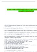
When the experimental manipulation is
carried out on the same entities => the
within-participant variance will be
made up of:
(1) The individual differences in
performance
AND
(2) The effect of the manipulation
The main difference with a repeated-measures design => look for the experimental effect
(SSM) within the individual – rather than within the group
, The only difference in sum of squares in repeated-measures => is where those SS come
from:
In repeated-measures => the model and the residual SS are both part of the within-
participant variance
The Total Sum of Squares, SST
In repeated-measures designs – the SS T is calculated in the same was as for one-way
independent designs
2
SS T =s grand ( N−1)
The grand variance => the variance of all scores when we ignore the group to which they
belong
The df for SST = N – 1
The Within-Participant Sum of Squares, SSW
The crucial difference from an independent design => in a repeated-measures design there is
a within-participant variance component
- i.e., represents individual differences within participants
In independent designs => these individual differences were quantified with the SSR
Because there are different participants within each condition => SS R within each
condition is calculated – and these values are added to get a total
In a repeated-measures design => different entities are subjected to more than one
experimental condition – and interested in the variation within an entity (not within a
condition)
Therefore, the same equation is used – but is adapted to look within participants:
SS W =s 2entity1 ( n1−1 ) + s 2entity 2 ( n 2−1 ) +s 2entity 3 ( n3−1 ) + …+ s 2entity n (nn−1)
(this chapter was ridiculously long so will post it by itself; chapters 16 and
17 will be posted asap)
Ch 15: Repeated-Measures Designs
Introduction to Repeated-Measures Designs
Between-subject designs => situations in which different entities contribute to different
means
Different people taking part in different experimental conditions
Repeated-Measures designs – i.e., within-subject designs – situations in which the same
entities contribute to different means
Repeated Measures => when the same entities participate in all conditions of an experiment
– or provide data at multiple time points
Testing the same people in all conditions of the experiment => allows to control for
individual differences
Repeated-Measures and the Linear Model
Conceptualizing a repeated-measures experiment as a linear model – cannot be done using
the same linear equation as has been used with the previous designs:
Y i=b0 +b1 X 1 i +ɛ i
This linear model => does not account for the fact that the same people took part in all
conditions
In an independent design => we have one observation for the outcome of each
participant
- Predicting the outcome for the individual based on the value of the predictor for
that person
,With repeated-measures => the participant has several values of the predictor:
The outcome is predicted from both the individual (i) and the specific value of the
predictor that is of interest (g)
Y gi =b0 +b 1 X g i +ɛ g i
The above equation => acknowledges that we predict the outcome from the predictor (g)
within the person (i) from the specific predictor that has been experienced by the participant (
X g i)
All that has changed is the subscripts in the model – which acknowledge that levels of the
treatment condition (g) occur within individuals (i)
Additionally => want to factor in that naturally there will be individual differences in regards
to the outcome
We do this by adding a variance term to the intercept (i.e., intercept represents the
value of the outcome, when the predictor = 0)
- By allowing this parameter to vary across individuals => effectively modeling the
possibility that different people will have different responses/reactions (individual
differences)
This is known as a random intercept model – written as:
Y gi =b0 +b 1 X g i +ɛ g i
b 0i =b0 +u 0i
The intercept has had a i added to the subscript => reflecting that it is specific to the
individual
Underneath => define the intercept as being made up of the group-level intercept ( b 0)
plus the deviation of the individual’s intercept from the group-level intercept (u0 i )
u0 i => reflects individual differences in the outcome
The first line of the equation => becomes a model for an individual; and the second line =>
the group-level effects
Additionally => factor in the possibility that the effect of different predictors varies across
individuals
, Add a variance term to the slope (i.e., the slope represents the effect that different
predictors have on the outcome)
- By allowing this parameter to vary across individuals => model the possibility
that the effect of the predictor on the outcome will be different in different
participants
This is known as a random slope model:
Y gi =b0 +b 1 X g i +ɛ g i
b 0i =b0 +u 0i
b 1i=b1 +u1 i
The main change is that the slope (b1) has had an i added to the subscript => reflecting that it
is specific to an individual
Defined as being made up of the group-level slope (b1) plus the deviation of the
individual’s slope from the group-level slope ( u1 i) => reflecting individual differences
in the effect of the predictor on the outcome
The top of the equation => a model for the individual; and bottom two lines => the group-
level effects
The ANOVA Approach to Repeated-Measures Designs
The Assumption of Sphericity
The assumption that allows the use of a simpler model to analyze repeated-measures data =>
known as sphericity
It is assuming that the relationship between scores in pairs of treatment conditions is
similar (i.e., the level of dependence between means is roughly equal)
It is denoted by ε – and referred to as circularity – it can be likened to the assumption
of homogeneity of variance in between-group designs
It is a form of compound symmetry => which holds true when both the variances across
conditions are equal – and the covariances between pairs of conditions are equal
, Assume that the variation within conditions is similar – and no two conditions are any
more dependent than any other two conditions
Sphericity => a more general, less restrictive form of compound symmetry
- Refers to the equality of variances of the differences between treatment levels
Example: if there were three conditions (A, B, and C)
Sphericity will hold when the variance of the differences between the different conditions is
similar:
variance A− B ≈ variance A −C ≈ varianceB −C
If two of the three group variances are very similar – then these data have local sphericity
- Sphericity can be assumed for any multiple comparisons involving these two
conditions
Assessing the Severity of Departures from Sphericity
Mauchly’s test => assess the hypothesis that the variances of the differences between
conditions are equal
If significant (i.e., the probability value < .05) => implies that there are significant
differences between the variances
- Sphericity is not met
If non-significant => the variances of differences are roughly equal and sphericity is
met
However – this test depends on sample size and is best ignored…
A better estimate of the degree of sphericity is the Greenhouse-Geisser estimate (ε^ ) => this
estimate varies between 1/(k – 1)
- Where k is the number of repeated-measures conditions
- E.g., when there are 5 conditions => the lower limit of ε^ will be 1(5 – 1); or 0.25
(i.e., the lower-bound estimate of sphericity)
Or use the Huynh-Feldt estimate (~ε )
, The Effect of Violating the Assumption of Sphericity
Sphericity creates a loss of power and an F-statistic that does not have the distribution it is
supposed to have (i.e., an F-distribution)
Lack of sphericity also causes complications for post hoc tests
When sphericity is violated => use the Bonferroni method as it is most robust in terms of
power and control of Type I error rate
When the assumption is definitely not violated => can use Tukey’s test
Steps to Take when Sphericity is Violated
Adjust the degrees of freedom of any F-statistic affected
Sphericity can be estimated in various of ways => resulting in a value = 1 when the data are
spherical – and a value < 1 when they are not
1. Multiple the degrees of freedom for an affected F-statistic by this estimate
2. The result is that when there is sphericity => the df will not change (as they’re
multiplied by 1)
3. When there is not sphericity => the df will get smaller (as they are multiplied by a
value less than 1)
The greater the violation of sphericity => the smaller the estimate gets => the smaller the
degrees of freedom become
Smaller degrees of freedom => make the p-value associated with the F-statistic less
significant
By adjusting the df – by the extent to which the data are not spherical => the F-statistic
becomes more conservative
This way => the Type I error is controlled
The df => adjusted using either the Greenhouse-Geisser or Huynh-Feldt estimates of
sphericity
, 1. When the Greenhouse-Geisser estimate > 0.75
- The correction is too conservative => this can be true when the sphericity estimate
is as high as 0.90
2. The Huynh-Feldt estimate => tends to overestimate sphericity
Recommended:
When estimates of sphericity > 0.75 => use the Huynh-Feldt estimate
When the Greenhouse-Geisser estimate of sphericity < 0.75 or nothing is known
about sphericity => use the GG correction
Suggested to take an average of the two estimates => and adjusting the df by this average
Another option is to use MANOVA => as it does not assume sphericity
- But there may be trade-offs in power
The F-Statistic for Repeated-Measures Designs
In a repeated-measures design => the effect of the experiment (i.e., the independent variable)
is show up in the Within-Participant variance (=> rather than the between-group variance)
In independent designs => the within-participant variance is the SSR (i.e., the variance
created by individual differences in performance)
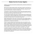
When the experimental manipulation is
carried out on the same entities => the
within-participant variance will be
made up of:
(1) The individual differences in
performance
AND
(2) The effect of the manipulation
The main difference with a repeated-measures design => look for the experimental effect
(SSM) within the individual – rather than within the group
, The only difference in sum of squares in repeated-measures => is where those SS come
from:
In repeated-measures => the model and the residual SS are both part of the within-
participant variance
The Total Sum of Squares, SST
In repeated-measures designs – the SS T is calculated in the same was as for one-way
independent designs
2
SS T =s grand ( N−1)
The grand variance => the variance of all scores when we ignore the group to which they
belong
The df for SST = N – 1
The Within-Participant Sum of Squares, SSW
The crucial difference from an independent design => in a repeated-measures design there is
a within-participant variance component
- i.e., represents individual differences within participants
In independent designs => these individual differences were quantified with the SSR
Because there are different participants within each condition => SS R within each
condition is calculated – and these values are added to get a total
In a repeated-measures design => different entities are subjected to more than one
experimental condition – and interested in the variation within an entity (not within a
condition)
Therefore, the same equation is used – but is adapted to look within participants:
SS W =s 2entity1 ( n1−1 ) + s 2entity 2 ( n 2−1 ) +s 2entity 3 ( n3−1 ) + …+ s 2entity n (nn−1)