CH3 Continuous Probability Distributions
To construct a random variable we start by listing all the outcomes of the
experiment under consideration in the sample space (Ω).
o then introduce a probability measure P(.) over Ω that must satisfy the
axioms of probability.
A random variable is defined as a function X :Ω → x where x ⊆ R (x is the
support of X).
To work with continuous random variables → perform basic integration.
Integration:
The following figure is the graphical representation of a function y = f (x ):
Consider the region A bounded by the function y = f (x) ≥ 0, the x-axis and the
vertical lines x = a and x = b, with a ≤ x ≤ b.
o Area of A is the definite integral btwn. limits x = a & x = b.
, The following integration results are NB
The probability density function
If X is a continuous random variable with sample space, Ω, and probability
density function (pdf), fX (x), the following is true:
To construct a random variable we start by listing all the outcomes of the
experiment under consideration in the sample space (Ω).
o then introduce a probability measure P(.) over Ω that must satisfy the
axioms of probability.
A random variable is defined as a function X :Ω → x where x ⊆ R (x is the
support of X).
To work with continuous random variables → perform basic integration.
Integration:
The following figure is the graphical representation of a function y = f (x ):
Consider the region A bounded by the function y = f (x) ≥ 0, the x-axis and the
vertical lines x = a and x = b, with a ≤ x ≤ b.
o Area of A is the definite integral btwn. limits x = a & x = b.
, The following integration results are NB
The probability density function
If X is a continuous random variable with sample space, Ω, and probability
density function (pdf), fX (x), the following is true: