Table of contents
Practical 1: Data import/export, data types and manipulation............................................................... 3
0. Before you start.................................................................................................................................. 3
1. Reading in a table .......................................................................................................................... 4
2. Data structure ............................................................................................................................... 6
3. Data types and coercion ................................................................................................................ 7
4. Making a new variable ................................................................................................................... 9
5. Exporting a modified table ........................................................................................................... 10
6. Indexing ...................................................................................................................................... 11
7. Sorting........................................................................................................................................ 14
8. Conditional selection .................................................................................................................. 15
9. Spitting, stacking and merging files............................................................................................... 19
10. Plotting in R (part1) .................................................................................................................. 20
11. Plotting in R (part 2) ................................................................................................................. 22
11.1 Plotting from a data frame ......................................................................................................... 22
11.2 Annotating a plot ...................................................................................................................... 24
11.3 Multipanel plots........................................................................................................................ 26
11.4 Exporting a graph ...................................................................................................................... 27
Practical 2 : Statistical analysis is R ................................................................................................... 28
1. Demo : the independent sample t-test .............................................................................................. 28
1.1 Data in long format : ozoneLong.txt ............................................................................................. 28
2. Parametric and non-parametric testing / Normality ............................................................................ 31
3. Simple linear regression ................................................................................................................... 32
3.1 Intro ........................................................................................................................................... 32
3.2 Fitting the model......................................................................................................................... 33
3.3 Graphical representation ............................................................................................................ 36
3.4 Model checks ............................................................................................................................. 36
4. Analysis of Variance (ANOVA) ........................................................................................................... 39
4.1 Intro ........................................................................................................................................... 39
4.2 Fitting the model......................................................................................................................... 39
4.3 More exploration and graphical representation ............................................................................. 44
Practical 3 - Part 1 - Automation in R : loops, lists and functions .......................................................... 47
1. Introduction ................................................................................................................................ 47
2. Automation 1: Looping ................................................................................................................ 47
3. Automation 2 : a new function ...................................................................................................... 54
4. Automation 3 : using a list ............................................................................................................ 57
1
, 5. Combining for-loops, functions and lists ....................................................................................... 58
Practical 3 - Part 2 - Data reshaping : Conversion long to wide format .................................................. 59
1. Introduction ................................................................................................................................ 59
2. Data reshaping............................................................................................................................ 59
3. Application : plotting growth using a line plot ................................................................................ 61
Principal 4: component analysis and cluster analysis......................................................................... 66
1. Principal components analysis (PCA) : the heptathlon dataset. ..................................................... 66
2. Cluster analysis: The wine dataset ............................................................................................... 76
3. Hierarchical cluster analysis ........................................................................................................ 77
4. Partitional clustering ................................................................................................................... 80
Practical 5: Multiple linear regression and linear mixed models .......................................................... 86
1. Multiple linear regression (ANCOVA model) .................................................................................. 86
1.1 Graphical analysis ...................................................................................................................... 87
1.2 Fitting the ANCOVA model .......................................................................................................... 89
1.3 Visualizing the ANCOVA model .................................................................................................... 92
2. Linear mixed model.......................................................................................................................... 94
2.1 Sketching the problem ................................................................................................................ 94
2.2 Fitting a linear mixed model......................................................................................................... 97
3. Longitudinal study with group:time interaction..................................................................................102
3.1 Introduction to the data ............................................................................................................ 102
3.2 Fitting the mixed model ............................................................................................................. 103
2
,Practical 1: Data import/export, data types and
manipulation
0. Before you start
For any analysis in R, it is good practice to create a working directory for your analysis .This
is the folder in which you collect your input files, you programming code (also called “the
script”), your output, correspondence…For this particular course, you can define a working
directory on a memory stick, or locally on the C-drive. In this manual, we made C:\temp our
working directory. Open RStudio by double-clicking on the icon. Create a new script file by :
File/New/Rscript
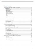
The screen is split into 4 quadrants:
1) The script editor (top left) : visualizing the script file with your R-commands. This is
comparable to the syntax window in SPSS or the script window in SAS.
In this text document, you can type your commands, execute them and save the script file for
later use. This is the file you will save after the analysis (in R, you typically save the code,
and not the output). R-script files is stored as a flat text file, that can be opened in
Notepad or WordPad.
To run the current line, hit CRTL+Enter - You can also run a selected block if the commands
span multiple lines
2) The command prompt (bottom left) : Here you can directly type in commands at the prompt.
Easy for a quick check or calculation that you don’t want to include into the code.
3) The workspace (top right) : This stores all objects you have defined (see later).
4) Output panel (bottom right) : Here you can see plots, look for help, select packages (see later)
The first thing we do is telling R what our working directory is. Using the getwd() command you
can see what the current working directory is:
getwd()
When opening R, make this C:\temp your home directory. One of the advantages is that you only
need to tell R the filename and not the entire path (saves typing!). To change the working directory,
go to Session/Set working directory/Choose directory and browse to the C:\temp. The
function setwd() does exactly the same thing (using forward slashes!):
setwd("C:/temp/whereverYourFilesAre")
Check that the working directory has changed
getwd()
Using the list.files() function, you can get an overview of the files that are in your working
directory list.files(getwd())
3
, 1. Reading in a table
Put the file DATA.xls into your working directory.
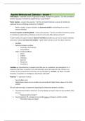
Open the DATA.xls workbook (in Excel). The data represent the results of an evaluation of two
statistics courses. Eight people completed one of three workshops, took exam and then filled out the
evaluation form. Columns E, F and G refer to the answer they gave on 3 of the questions (scale 1 to
5). The last column shows the mean of these 3 latter scores.
The table is quite messy. Scan for expressions/characters that have to be avoided and remove these.
• ? = missing value (person did not fill in this information) à recognized as text character by R
o Should be filled in as NA (recognized by default)
• Text of gender is seen as a character and not a factor
• Decimal number “.” Or “,” but may not be combined à specification needed otherwise R
recognized “,’ as a character and not as a calculation factor
• Every column has to have a header or none (first row)
o Needs to be manually fixed eg. Write ID in top left column
o Cannot be solved by R
• A space in eg. Names are recognized as column dilinears
o Eg. Van Persie à van = column 1 and persie = column 2
• The space between “question” and “1” has to be removed
• Brackets in header: can nowadays be read by R, but is changed into a “.”
o Header should start with a letter and can only have letters, numbers and underscores
o So in the last header remove the “(,)” brackets
• Functions are nowadays also recognized by R
• Empty cells should be avoided
After you finished your editing, save the excel workbook.
To create a tab-delimited (.txt) file, go to
File\ save as\ …
Save as type text (Tab delimited)(.txt).
You get a warning that the document may contain features not compatible with the .txt format, and
that you are only saving the active sheet. Click OK/yes. Quit the excel workbook without further
saving (you already did save your workbook before).
In your directory, check if the .txt document has been created. Open the document (in notepad) by
double clicking. Check that the columns are separated by tabs. What happened to the white spaces in
the first column?
The R-function to read in the table is… read.table().At the command prompt (bottom left panel),
ask for help on the read.table() function by typing ?read.table. The help file lists all possible
arguments, along with their defaults. Additional explanation on each argument is supplied in the
‘Arguments’ section of the help file.
The first argument is the file. If you have assigned your working directory, the name of the file alone
is sufficient.
read.table(file = "data.txt",…) # don’t run this yet! See below why!
4
,Since our file does have column headers, we have to supply the argument header=TRUE.
read.table(file = "data.txt",header=TRUE) # Not sufficient yet!
In addition, we must specify that columns with text strings are read in as factors
read.table(file = "data.txt",header=TRUE, stringsAsFactors=TRUE)
# Still Not sufficient yet!
Search further for the defaults on missing data, decimal separation, and separators.
The first column contains strings with a white space (Van Persie). These white spaces are erroneously
used as field separator. We need to tell R that only tabs should be used to separate columns.
Add the following argument to the read.table() command
sep="\t"
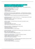
Now the file gets read in. It pops up onto the screen. You can assign this table to an R-object. In
the remainder of this handout, this object is called “myData”
myData <- read.table(file="data1.txt",sep="\t",header=T)
No output is shown on the screen now, but the object “myData” is now stored in your workspace.
You can see the object “myData” appear in the top right panel of R Studio.
• When you tab on the blue arrow à it tells you what the different variables look like
and how you read in those
Type the word “myData” at the prompt (bottom left panel in RStudio) and see what happens.
Remember, R is case sensitive!! “myData” is not the same as “MYDATA” or “mydata”!!
Conclusie: read.table("DATA.txt",header=TRUE,sep="\t",dec=".",na.strings="?",stringsAsFactors =
TRUE)
• Header = true à we indicate that the first line of our inputdata contains the variable names
• Sep = ="\t" à columns are separated with tabs
• Dec = “,” à file is using “,” the European way
• Na.strings = “?” à missing value indicates as NA
5
, 2. Data structure
• You have different types of variables
• Organization of variables into data structures
Using the assignment operator (<-), you have given a name to the data you’ve read in.
myData <- read.table("data1.txt",… )
This has created the object “myData”. It appears in the top right panel of RStudio.
Whenever you now use the word ‘myData’, in a formula or a calculation, R knows that it
stands for the particular data structure you just read in. What kind of data structure would it be? Use
the class function.
class(myData)
myData is an object of class “data frame”. Objects of class data frame represent data the traditional
table, with each row consisting of a single observation and the variables are arranged into columns.
The variables can be of different types. A more comprehensive overview of the current data structure
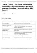
is given by the str() function
str(myData)
The output tells you again that ‘myData’ is an object of class data frame, how many
observations and variables, and what type of data the different variables represent.
In R, the names of the variables are an entire part of the data frame. They can be invoked using the
names function.
names(myData)
The output of this command is a character vector: a 1-dimensional matrix, of which every element is
a character string.
The dimensions of a table can be extracted using the dim function
dim(myData)
Alternatively, the number of rows and columns can be found using:
nrow(myData)
ncol(myData)
CONCLUSIE:
6
Practical 1: Data import/export, data types and manipulation............................................................... 3
0. Before you start.................................................................................................................................. 3
1. Reading in a table .......................................................................................................................... 4
2. Data structure ............................................................................................................................... 6
3. Data types and coercion ................................................................................................................ 7
4. Making a new variable ................................................................................................................... 9
5. Exporting a modified table ........................................................................................................... 10
6. Indexing ...................................................................................................................................... 11
7. Sorting........................................................................................................................................ 14
8. Conditional selection .................................................................................................................. 15
9. Spitting, stacking and merging files............................................................................................... 19
10. Plotting in R (part1) .................................................................................................................. 20
11. Plotting in R (part 2) ................................................................................................................. 22
11.1 Plotting from a data frame ......................................................................................................... 22
11.2 Annotating a plot ...................................................................................................................... 24
11.3 Multipanel plots........................................................................................................................ 26
11.4 Exporting a graph ...................................................................................................................... 27
Practical 2 : Statistical analysis is R ................................................................................................... 28
1. Demo : the independent sample t-test .............................................................................................. 28
1.1 Data in long format : ozoneLong.txt ............................................................................................. 28
2. Parametric and non-parametric testing / Normality ............................................................................ 31
3. Simple linear regression ................................................................................................................... 32
3.1 Intro ........................................................................................................................................... 32
3.2 Fitting the model......................................................................................................................... 33
3.3 Graphical representation ............................................................................................................ 36
3.4 Model checks ............................................................................................................................. 36
4. Analysis of Variance (ANOVA) ........................................................................................................... 39
4.1 Intro ........................................................................................................................................... 39
4.2 Fitting the model......................................................................................................................... 39
4.3 More exploration and graphical representation ............................................................................. 44
Practical 3 - Part 1 - Automation in R : loops, lists and functions .......................................................... 47
1. Introduction ................................................................................................................................ 47
2. Automation 1: Looping ................................................................................................................ 47
3. Automation 2 : a new function ...................................................................................................... 54
4. Automation 3 : using a list ............................................................................................................ 57
1
, 5. Combining for-loops, functions and lists ....................................................................................... 58
Practical 3 - Part 2 - Data reshaping : Conversion long to wide format .................................................. 59
1. Introduction ................................................................................................................................ 59
2. Data reshaping............................................................................................................................ 59
3. Application : plotting growth using a line plot ................................................................................ 61
Principal 4: component analysis and cluster analysis......................................................................... 66
1. Principal components analysis (PCA) : the heptathlon dataset. ..................................................... 66
2. Cluster analysis: The wine dataset ............................................................................................... 76
3. Hierarchical cluster analysis ........................................................................................................ 77
4. Partitional clustering ................................................................................................................... 80
Practical 5: Multiple linear regression and linear mixed models .......................................................... 86
1. Multiple linear regression (ANCOVA model) .................................................................................. 86
1.1 Graphical analysis ...................................................................................................................... 87
1.2 Fitting the ANCOVA model .......................................................................................................... 89
1.3 Visualizing the ANCOVA model .................................................................................................... 92
2. Linear mixed model.......................................................................................................................... 94
2.1 Sketching the problem ................................................................................................................ 94
2.2 Fitting a linear mixed model......................................................................................................... 97
3. Longitudinal study with group:time interaction..................................................................................102
3.1 Introduction to the data ............................................................................................................ 102
3.2 Fitting the mixed model ............................................................................................................. 103
2
,Practical 1: Data import/export, data types and
manipulation
0. Before you start
For any analysis in R, it is good practice to create a working directory for your analysis .This
is the folder in which you collect your input files, you programming code (also called “the
script”), your output, correspondence…For this particular course, you can define a working
directory on a memory stick, or locally on the C-drive. In this manual, we made C:\temp our
working directory. Open RStudio by double-clicking on the icon. Create a new script file by :
File/New/Rscript
The screen is split into 4 quadrants:
1) The script editor (top left) : visualizing the script file with your R-commands. This is
comparable to the syntax window in SPSS or the script window in SAS.
In this text document, you can type your commands, execute them and save the script file for
later use. This is the file you will save after the analysis (in R, you typically save the code,
and not the output). R-script files is stored as a flat text file, that can be opened in
Notepad or WordPad.
To run the current line, hit CRTL+Enter - You can also run a selected block if the commands
span multiple lines
2) The command prompt (bottom left) : Here you can directly type in commands at the prompt.
Easy for a quick check or calculation that you don’t want to include into the code.
3) The workspace (top right) : This stores all objects you have defined (see later).
4) Output panel (bottom right) : Here you can see plots, look for help, select packages (see later)
The first thing we do is telling R what our working directory is. Using the getwd() command you
can see what the current working directory is:
getwd()
When opening R, make this C:\temp your home directory. One of the advantages is that you only
need to tell R the filename and not the entire path (saves typing!). To change the working directory,
go to Session/Set working directory/Choose directory and browse to the C:\temp. The
function setwd() does exactly the same thing (using forward slashes!):
setwd("C:/temp/whereverYourFilesAre")
Check that the working directory has changed
getwd()
Using the list.files() function, you can get an overview of the files that are in your working
directory list.files(getwd())
3
, 1. Reading in a table
Put the file DATA.xls into your working directory.
Open the DATA.xls workbook (in Excel). The data represent the results of an evaluation of two
statistics courses. Eight people completed one of three workshops, took exam and then filled out the
evaluation form. Columns E, F and G refer to the answer they gave on 3 of the questions (scale 1 to
5). The last column shows the mean of these 3 latter scores.
The table is quite messy. Scan for expressions/characters that have to be avoided and remove these.
• ? = missing value (person did not fill in this information) à recognized as text character by R
o Should be filled in as NA (recognized by default)
• Text of gender is seen as a character and not a factor
• Decimal number “.” Or “,” but may not be combined à specification needed otherwise R
recognized “,’ as a character and not as a calculation factor
• Every column has to have a header or none (first row)
o Needs to be manually fixed eg. Write ID in top left column
o Cannot be solved by R
• A space in eg. Names are recognized as column dilinears
o Eg. Van Persie à van = column 1 and persie = column 2
• The space between “question” and “1” has to be removed
• Brackets in header: can nowadays be read by R, but is changed into a “.”
o Header should start with a letter and can only have letters, numbers and underscores
o So in the last header remove the “(,)” brackets
• Functions are nowadays also recognized by R
• Empty cells should be avoided
After you finished your editing, save the excel workbook.
To create a tab-delimited (.txt) file, go to
File\ save as\ …
Save as type text (Tab delimited)(.txt).
You get a warning that the document may contain features not compatible with the .txt format, and
that you are only saving the active sheet. Click OK/yes. Quit the excel workbook without further
saving (you already did save your workbook before).
In your directory, check if the .txt document has been created. Open the document (in notepad) by
double clicking. Check that the columns are separated by tabs. What happened to the white spaces in
the first column?
The R-function to read in the table is… read.table().At the command prompt (bottom left panel),
ask for help on the read.table() function by typing ?read.table. The help file lists all possible
arguments, along with their defaults. Additional explanation on each argument is supplied in the
‘Arguments’ section of the help file.
The first argument is the file. If you have assigned your working directory, the name of the file alone
is sufficient.
read.table(file = "data.txt",…) # don’t run this yet! See below why!
4
,Since our file does have column headers, we have to supply the argument header=TRUE.
read.table(file = "data.txt",header=TRUE) # Not sufficient yet!
In addition, we must specify that columns with text strings are read in as factors
read.table(file = "data.txt",header=TRUE, stringsAsFactors=TRUE)
# Still Not sufficient yet!
Search further for the defaults on missing data, decimal separation, and separators.
The first column contains strings with a white space (Van Persie). These white spaces are erroneously
used as field separator. We need to tell R that only tabs should be used to separate columns.
Add the following argument to the read.table() command
sep="\t"
Now the file gets read in. It pops up onto the screen. You can assign this table to an R-object. In
the remainder of this handout, this object is called “myData”
myData <- read.table(file="data1.txt",sep="\t",header=T)
No output is shown on the screen now, but the object “myData” is now stored in your workspace.
You can see the object “myData” appear in the top right panel of R Studio.
• When you tab on the blue arrow à it tells you what the different variables look like
and how you read in those
Type the word “myData” at the prompt (bottom left panel in RStudio) and see what happens.
Remember, R is case sensitive!! “myData” is not the same as “MYDATA” or “mydata”!!
Conclusie: read.table("DATA.txt",header=TRUE,sep="\t",dec=".",na.strings="?",stringsAsFactors =
TRUE)
• Header = true à we indicate that the first line of our inputdata contains the variable names
• Sep = ="\t" à columns are separated with tabs
• Dec = “,” à file is using “,” the European way
• Na.strings = “?” à missing value indicates as NA
5
, 2. Data structure
• You have different types of variables
• Organization of variables into data structures
Using the assignment operator (<-), you have given a name to the data you’ve read in.
myData <- read.table("data1.txt",… )
This has created the object “myData”. It appears in the top right panel of RStudio.
Whenever you now use the word ‘myData’, in a formula or a calculation, R knows that it
stands for the particular data structure you just read in. What kind of data structure would it be? Use
the class function.
class(myData)
myData is an object of class “data frame”. Objects of class data frame represent data the traditional
table, with each row consisting of a single observation and the variables are arranged into columns.
The variables can be of different types. A more comprehensive overview of the current data structure
is given by the str() function
str(myData)
The output tells you again that ‘myData’ is an object of class data frame, how many
observations and variables, and what type of data the different variables represent.
In R, the names of the variables are an entire part of the data frame. They can be invoked using the
names function.
names(myData)
The output of this command is a character vector: a 1-dimensional matrix, of which every element is
a character string.
The dimensions of a table can be extracted using the dim function
dim(myData)
Alternatively, the number of rows and columns can be found using:
nrow(myData)
ncol(myData)
CONCLUSIE:
6