Green’s Theorem
Green’s theorem is a generalization of the fundamental theorem of Calculus:
𝑏
∫𝑎 𝑓 ′ (𝑥 )𝑑𝑥 = 𝑓(𝑏) − 𝑓(𝑎 ).
Notice that the FTC relates the definite integral of 𝑓 ′ (𝑥) over a line segment, [𝑎, 𝑏],
with the value of the function 𝑓 (𝑥) at the endpoints of that interval (i.e. at a and b).
Another way to think of the endpoints of an interval (i.e., a line segment) is as the
boundary of that interval (much the way the unit circle is the boundary of the unit
disk, 𝑥 2 + 𝑦 2 ≤ 1). So the FTC relates the definite integral of 𝑓 ′ (𝑥) over a line
segment with the value of the function 𝑓 (𝑥) on the boundary of the interval.
Green’s theorem relates a double integral of a function (we will see later how this
function is similar to the “derivative” of another function) over an elementary region
in ℝ2 with a line integral around the boundary of that region.
Green’s Theorem: Let 𝐷 be a simple region and let 𝑐 be its boundary. Suppose
𝑃: 𝐷 → ℝ and 𝑄: 𝐷 → ℝ are both 𝐶 1 functions then
𝜕𝑄 𝜕𝑃
∫𝑐 𝑃(𝑥, 𝑦)𝑑𝑥 + 𝑄 (𝑥, 𝑦)𝑑𝑦 = ∬𝐷 ( 𝜕𝑥 − 𝜕𝑦)𝑑𝑥𝑑𝑦.
Note: We denote the “boundary of 𝐷” by 𝜕𝐷, so we could rewrite Green’s thm as:
𝜕𝑄 𝜕𝑃
∫𝜕𝐷 𝑃(𝑥, 𝑦)𝑑𝑥 + 𝑄 (𝑥, 𝑦)𝑑𝑦 = ∬𝐷 ( 𝜕𝑥 − 𝜕𝑦)𝑑𝑥𝑑𝑦.
Green’s theorem is useful because sometimes one side of Green’s theorem is
much easier to evaluate than the other side.
, 2
We can prove Green’s theorem by proving the following two lemmas.
Lemma 1: Let 𝐷 be a 𝑦-simple region and let 𝑐 = 𝜕𝐷. Suppose 𝑃: 𝐷 → ℝ is of class
𝜕𝑃
𝐶 1 then: ∫𝑐 𝑃(𝑥, 𝑦)𝑑𝑥 = − ∬𝐷 𝜕𝑦
𝑑𝑥𝑑𝑦.
Lemma 2: Let 𝐷 be an 𝑥-simple region and let 𝑐 = 𝜕𝐷. Suppose 𝑄: 𝐷 → ℝ is of class
𝜕𝑄
𝐶 1 then: ∫𝑐 𝑄(𝑥, 𝑦)𝑑𝑥 = ∬𝐷 𝜕𝑥
𝑑𝑥𝑑𝑦.
Adding the conclusions to lemma 1 and lemma 2 gives Green’s theorem.
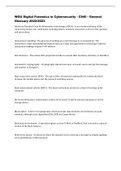
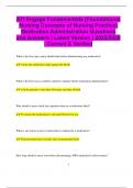
To prove lemma 1 let’s assume that 𝐷 is bounded below by the curve 𝑦 = 𝑓(𝑥),
above by the curve 𝑦 = 𝑔(𝑥) and on the sides by 𝑥 = 𝑎 and 𝑥 = 𝑏.
𝜕𝐷 = 𝑐 = 𝑐1 + 𝑐2 − 𝑐3 − 𝑐4 (oriented counterclockwise) where
𝑦 = 𝑔(𝑥)) 𝑐3
𝑐⃗1 (𝑡 ) =< 𝑡, 𝑓(𝑡 ) > : 𝑎 ≤ 𝑡 ≤ 𝑏
𝑐4 𝑐2
𝐷 𝑐⃗2 (𝑡 ) =< 𝑏, 𝑡 >; 𝑓(𝑏) ≤ 𝑡 ≤ 𝑔(𝑏)
𝑐1
𝑦 = 𝑓(𝑥) 𝑐⃗3 (𝑡 ) =< 𝑡, 𝑔(𝑡 ) >; 𝑎≤𝑡≤𝑏
𝑎 𝑏 𝑐⃗4 (𝑡 ) =< 𝑎, 𝑡 >; 𝑓(𝑎) ≤ 𝑡 ≤ 𝑔(𝑎).
By Fubini’s theorem we can say:
𝜕𝑃 𝑥=𝑏 𝑦=𝑔(𝑥) 𝜕𝑃
∬𝐷 𝑑𝑥𝑑𝑦 = ∫𝑥=𝑎 [∫𝑦=𝑓(𝑥) 𝑑𝑦]𝑑𝑥 .
𝜕𝑦 𝜕𝑦
Now by the fundamental theorem of Calculus we have:
𝜕𝑃 𝑥=𝑏
∬𝐷 𝑑𝑥𝑑𝑦 = ∫𝑥=𝑎 [𝑃(𝑥, 𝑔(𝑥 )) − 𝑃(𝑥, 𝑓(𝑥 ))]𝑑𝑥 .
𝜕𝑦
Now let’s evaluate the line integral around 𝜕𝐷 = 𝑐:
𝑡=𝑏 𝑡=𝑏
∫𝑐 𝑃(𝑥, 𝑦)𝑑𝑥 = ∫𝑡=𝑎 𝑃(𝑡, 𝑓 (𝑡 ))𝑑𝑡 − ∫𝑡=𝑎 𝑃(𝑡, 𝑔(𝑡 ))𝑑𝑡.
, 3
𝑑𝑥
Notice that the line integrals along 𝑐2 and 𝑐4 are both 0 because = 0.
𝑑𝑡
If we rewrite this line integral around 𝑐, replacing 𝑥 for 𝑡 we get:
𝑥=𝑏
∫𝑐 𝑃(𝑥, 𝑦)𝑑𝑥 = ∫𝑥=𝑎 [𝑃(𝑥, 𝑓 (𝑥)) − 𝑃(𝑥, 𝑔(𝑥))]𝑑𝑥
𝑥=𝑏
= − ∫𝑥=𝑎 [𝑃(𝑥, 𝑔(𝑥)) − 𝑃(𝑥, 𝑓(𝑥))]𝑑𝑥.
𝜕𝑃
Now notice from our earlier calculation for ∬𝐷 𝑑𝑥𝑑𝑦 we have:
𝜕𝑦
𝜕𝑃
∫𝑐 𝑃(𝑥, 𝑦)𝑑𝑥 = − ∬𝐷 𝜕𝑦
𝑑𝑥𝑑𝑦.
A similar argument also proves lemma 2.
Ex. Evaluate ∫𝑐 (3𝑦 − 𝑒 𝑠𝑖𝑛𝑥 )𝑑𝑥 + (7𝑥 + √𝑦 4 + 1)𝑑𝑦; where c is the circle
𝑥 2 + 𝑦 2 = 9 oriented counterclockwise.
Suppose we just try to evaluate this line integral directly.
𝑥 = 3cost, y = 3sint; dx = (−3sint)dt, dy = (3cost)dt.
So the line integral becomes:
2𝜋
∫ (9𝑠𝑖𝑛𝑡 − 𝑒 sin(3𝑐𝑜𝑠𝑡) )(−3𝑠𝑖𝑛𝑡 )𝑑𝑡 + (21𝑐𝑜𝑠𝑡 + √81𝑠𝑖𝑛4 𝑡 + 1)(3𝑐𝑜𝑠𝑡)𝑑𝑡
0
Ugh!!!
Green’s theorem is a generalization of the fundamental theorem of Calculus:
𝑏
∫𝑎 𝑓 ′ (𝑥 )𝑑𝑥 = 𝑓(𝑏) − 𝑓(𝑎 ).
Notice that the FTC relates the definite integral of 𝑓 ′ (𝑥) over a line segment, [𝑎, 𝑏],
with the value of the function 𝑓 (𝑥) at the endpoints of that interval (i.e. at a and b).
Another way to think of the endpoints of an interval (i.e., a line segment) is as the
boundary of that interval (much the way the unit circle is the boundary of the unit
disk, 𝑥 2 + 𝑦 2 ≤ 1). So the FTC relates the definite integral of 𝑓 ′ (𝑥) over a line
segment with the value of the function 𝑓 (𝑥) on the boundary of the interval.
Green’s theorem relates a double integral of a function (we will see later how this
function is similar to the “derivative” of another function) over an elementary region
in ℝ2 with a line integral around the boundary of that region.
Green’s Theorem: Let 𝐷 be a simple region and let 𝑐 be its boundary. Suppose
𝑃: 𝐷 → ℝ and 𝑄: 𝐷 → ℝ are both 𝐶 1 functions then
𝜕𝑄 𝜕𝑃
∫𝑐 𝑃(𝑥, 𝑦)𝑑𝑥 + 𝑄 (𝑥, 𝑦)𝑑𝑦 = ∬𝐷 ( 𝜕𝑥 − 𝜕𝑦)𝑑𝑥𝑑𝑦.
Note: We denote the “boundary of 𝐷” by 𝜕𝐷, so we could rewrite Green’s thm as:
𝜕𝑄 𝜕𝑃
∫𝜕𝐷 𝑃(𝑥, 𝑦)𝑑𝑥 + 𝑄 (𝑥, 𝑦)𝑑𝑦 = ∬𝐷 ( 𝜕𝑥 − 𝜕𝑦)𝑑𝑥𝑑𝑦.
Green’s theorem is useful because sometimes one side of Green’s theorem is
much easier to evaluate than the other side.
, 2
We can prove Green’s theorem by proving the following two lemmas.
Lemma 1: Let 𝐷 be a 𝑦-simple region and let 𝑐 = 𝜕𝐷. Suppose 𝑃: 𝐷 → ℝ is of class
𝜕𝑃
𝐶 1 then: ∫𝑐 𝑃(𝑥, 𝑦)𝑑𝑥 = − ∬𝐷 𝜕𝑦
𝑑𝑥𝑑𝑦.
Lemma 2: Let 𝐷 be an 𝑥-simple region and let 𝑐 = 𝜕𝐷. Suppose 𝑄: 𝐷 → ℝ is of class
𝜕𝑄
𝐶 1 then: ∫𝑐 𝑄(𝑥, 𝑦)𝑑𝑥 = ∬𝐷 𝜕𝑥
𝑑𝑥𝑑𝑦.
Adding the conclusions to lemma 1 and lemma 2 gives Green’s theorem.
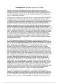
To prove lemma 1 let’s assume that 𝐷 is bounded below by the curve 𝑦 = 𝑓(𝑥),
above by the curve 𝑦 = 𝑔(𝑥) and on the sides by 𝑥 = 𝑎 and 𝑥 = 𝑏.
𝜕𝐷 = 𝑐 = 𝑐1 + 𝑐2 − 𝑐3 − 𝑐4 (oriented counterclockwise) where
𝑦 = 𝑔(𝑥)) 𝑐3
𝑐⃗1 (𝑡 ) =< 𝑡, 𝑓(𝑡 ) > : 𝑎 ≤ 𝑡 ≤ 𝑏
𝑐4 𝑐2
𝐷 𝑐⃗2 (𝑡 ) =< 𝑏, 𝑡 >; 𝑓(𝑏) ≤ 𝑡 ≤ 𝑔(𝑏)
𝑐1
𝑦 = 𝑓(𝑥) 𝑐⃗3 (𝑡 ) =< 𝑡, 𝑔(𝑡 ) >; 𝑎≤𝑡≤𝑏
𝑎 𝑏 𝑐⃗4 (𝑡 ) =< 𝑎, 𝑡 >; 𝑓(𝑎) ≤ 𝑡 ≤ 𝑔(𝑎).
By Fubini’s theorem we can say:
𝜕𝑃 𝑥=𝑏 𝑦=𝑔(𝑥) 𝜕𝑃
∬𝐷 𝑑𝑥𝑑𝑦 = ∫𝑥=𝑎 [∫𝑦=𝑓(𝑥) 𝑑𝑦]𝑑𝑥 .
𝜕𝑦 𝜕𝑦
Now by the fundamental theorem of Calculus we have:
𝜕𝑃 𝑥=𝑏
∬𝐷 𝑑𝑥𝑑𝑦 = ∫𝑥=𝑎 [𝑃(𝑥, 𝑔(𝑥 )) − 𝑃(𝑥, 𝑓(𝑥 ))]𝑑𝑥 .
𝜕𝑦
Now let’s evaluate the line integral around 𝜕𝐷 = 𝑐:
𝑡=𝑏 𝑡=𝑏
∫𝑐 𝑃(𝑥, 𝑦)𝑑𝑥 = ∫𝑡=𝑎 𝑃(𝑡, 𝑓 (𝑡 ))𝑑𝑡 − ∫𝑡=𝑎 𝑃(𝑡, 𝑔(𝑡 ))𝑑𝑡.
, 3
𝑑𝑥
Notice that the line integrals along 𝑐2 and 𝑐4 are both 0 because = 0.
𝑑𝑡
If we rewrite this line integral around 𝑐, replacing 𝑥 for 𝑡 we get:
𝑥=𝑏
∫𝑐 𝑃(𝑥, 𝑦)𝑑𝑥 = ∫𝑥=𝑎 [𝑃(𝑥, 𝑓 (𝑥)) − 𝑃(𝑥, 𝑔(𝑥))]𝑑𝑥
𝑥=𝑏
= − ∫𝑥=𝑎 [𝑃(𝑥, 𝑔(𝑥)) − 𝑃(𝑥, 𝑓(𝑥))]𝑑𝑥.
𝜕𝑃
Now notice from our earlier calculation for ∬𝐷 𝑑𝑥𝑑𝑦 we have:
𝜕𝑦
𝜕𝑃
∫𝑐 𝑃(𝑥, 𝑦)𝑑𝑥 = − ∬𝐷 𝜕𝑦
𝑑𝑥𝑑𝑦.
A similar argument also proves lemma 2.
Ex. Evaluate ∫𝑐 (3𝑦 − 𝑒 𝑠𝑖𝑛𝑥 )𝑑𝑥 + (7𝑥 + √𝑦 4 + 1)𝑑𝑦; where c is the circle
𝑥 2 + 𝑦 2 = 9 oriented counterclockwise.
Suppose we just try to evaluate this line integral directly.
𝑥 = 3cost, y = 3sint; dx = (−3sint)dt, dy = (3cost)dt.
So the line integral becomes:
2𝜋
∫ (9𝑠𝑖𝑛𝑡 − 𝑒 sin(3𝑐𝑜𝑠𝑡) )(−3𝑠𝑖𝑛𝑡 )𝑑𝑡 + (21𝑐𝑜𝑠𝑡 + √81𝑠𝑖𝑛4 𝑡 + 1)(3𝑐𝑜𝑠𝑡)𝑑𝑡
0
Ugh!!!