Populations and Systems Ecology CSA20806
Tutorial 1 – Exponential and Geometric Growth
The change in a population can be described as:
∆ N =B−D+ I −E
(N = number of individuals, B = birth, D = death, I = immigration,
E = emigration).
Geometric growth
Discrete time = time in steps.
N k ∆ t =λ k N 0
λ = net reproductive factor, has a ratio, no
dimension, the value depends on the size of
the time step.
k = number of time steps.
N0 = the initial number of individuals.
Exponential growth
Continuous time.
dN
=rN
dt
N = number of individuals
t = time
dN/dt = growth rate
r = intrinsic growth rate of the population,
dimension: t-1
Relation between r and λ:
ln ( λ )=r Δt
λ=e r Δt
ln ( λ )
r=
Δt
Discrete modelling Continuous modelling
Geometric growth Exponential growth
No changes during time step Continuous change
λ, net reproductive factor, dimensionless r, intrinsic growth rate, t-1
Difference equation Differential equation
N t +∆ t =λ N t dN
=rN
dt
N k ∆ t =λ k N 0 N t =N 0 e rt
,Tutorial 2 – Dynamics of Age-Structure Populations
A life table gives a compact summary of the average course of life with respect to ageing, survival
and reproduction. With a life table, calculations can be made to predict the development of a field
population. Data for the table can be gathered under natural or artificial conditions. Females are
usually used (for both parent-individuals and offspring) because they are the reproductive section of
a population.
Day Mothers Fraction Number of Number of
surviving offspring offspring per
mothers produced per living mother
day per day
Symbol x nx lx mx
Dimension (d) (#) (-) (#d-1) (##-1d-1)
Formula for survival fraction:
nx
lx =
n0
n0 = number of individuals at x = 0.
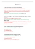
Survivorship curve: the evolution of the fraction survival in time.
3 standard types of survivorship curve:
Type 1 mortality is restricted to the last
phase of life (e.g. humans).
Type 2 the relative mortality in each phase of
life is the same (e.g. birds).
Type 3 large mortality occurs during the
juvenile stage (e.g. fish, parasites).
More possible expansions of a life table:
The number of individuals that dies during the interval (dx): d x =n x −n x+1
The life expectancy of the individuals that are present (ex):
1
ex= ( n +n +… etc …+ nk ) +∆ t where k is the highest age that can be reached.
n x x+1 x+2
k
Net replacement (R0) = the number of daughters R0 =∑ l x m x
x=0
Generation time (T) = the average time it takes for a new-born individual to produce new offspring
T=
∑ x l x mx
R0
, The equation for the calculation of the intrinsic growth rate r (only approximation (benadering)):
ln ( R0 )
r= .
T
Tutorial 3 – Leslie matrices (Age- and stage structured population
dynamics as a matrix process)
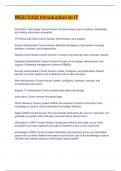
The parameters in the life cycle diagram can be organized into a Leslie Matrix:
0 9 12
)( )
f1 f2 f3 1
L= p1
0 ( 0
p2
0 = 3
0 0
0
1
2
0
0
Matrices can be multiplied with vectors.
Population dynamics can be based on different criterions, such as size or stage structured
populations, which are a little more complicated that age structured population dynamics.
The life cycle diagram and matrix A is for age
structured population dynamics. B and C are for
stage structured dynamics.
P = probabilities of survival.
F = fecundity, sexual reproduction.
G = growth.
A matrix for stage structured population dynamics
is sometimes called a Lefkovitch matrix, to
distinguish it from age-structured population
dynamics of a Leslie matrix. But the term Leslie
matrix is often used to encompass both age and
stage structured population dynamics.
Tutorial 1 – Exponential and Geometric Growth
The change in a population can be described as:
∆ N =B−D+ I −E
(N = number of individuals, B = birth, D = death, I = immigration,
E = emigration).
Geometric growth
Discrete time = time in steps.
N k ∆ t =λ k N 0
λ = net reproductive factor, has a ratio, no
dimension, the value depends on the size of
the time step.
k = number of time steps.
N0 = the initial number of individuals.
Exponential growth
Continuous time.
dN
=rN
dt
N = number of individuals
t = time
dN/dt = growth rate
r = intrinsic growth rate of the population,
dimension: t-1
Relation between r and λ:
ln ( λ )=r Δt
λ=e r Δt
ln ( λ )
r=
Δt
Discrete modelling Continuous modelling
Geometric growth Exponential growth
No changes during time step Continuous change
λ, net reproductive factor, dimensionless r, intrinsic growth rate, t-1
Difference equation Differential equation
N t +∆ t =λ N t dN
=rN
dt
N k ∆ t =λ k N 0 N t =N 0 e rt
,Tutorial 2 – Dynamics of Age-Structure Populations
A life table gives a compact summary of the average course of life with respect to ageing, survival
and reproduction. With a life table, calculations can be made to predict the development of a field
population. Data for the table can be gathered under natural or artificial conditions. Females are
usually used (for both parent-individuals and offspring) because they are the reproductive section of
a population.
Day Mothers Fraction Number of Number of
surviving offspring offspring per
mothers produced per living mother
day per day
Symbol x nx lx mx
Dimension (d) (#) (-) (#d-1) (##-1d-1)
Formula for survival fraction:
nx
lx =
n0
n0 = number of individuals at x = 0.
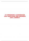
Survivorship curve: the evolution of the fraction survival in time.
3 standard types of survivorship curve:
Type 1 mortality is restricted to the last
phase of life (e.g. humans).
Type 2 the relative mortality in each phase of
life is the same (e.g. birds).
Type 3 large mortality occurs during the
juvenile stage (e.g. fish, parasites).
More possible expansions of a life table:
The number of individuals that dies during the interval (dx): d x =n x −n x+1
The life expectancy of the individuals that are present (ex):
1
ex= ( n +n +… etc …+ nk ) +∆ t where k is the highest age that can be reached.
n x x+1 x+2
k
Net replacement (R0) = the number of daughters R0 =∑ l x m x
x=0
Generation time (T) = the average time it takes for a new-born individual to produce new offspring
T=
∑ x l x mx
R0
, The equation for the calculation of the intrinsic growth rate r (only approximation (benadering)):
ln ( R0 )
r= .
T
Tutorial 3 – Leslie matrices (Age- and stage structured population
dynamics as a matrix process)
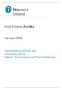
The parameters in the life cycle diagram can be organized into a Leslie Matrix:
0 9 12
)( )
f1 f2 f3 1
L= p1
0 ( 0
p2
0 = 3
0 0
0
1
2
0
0
Matrices can be multiplied with vectors.
Population dynamics can be based on different criterions, such as size or stage structured
populations, which are a little more complicated that age structured population dynamics.
The life cycle diagram and matrix A is for age
structured population dynamics. B and C are for
stage structured dynamics.
P = probabilities of survival.
F = fecundity, sexual reproduction.
G = growth.
A matrix for stage structured population dynamics
is sometimes called a Lefkovitch matrix, to
distinguish it from age-structured population
dynamics of a Leslie matrix. But the term Leslie
matrix is often used to encompass both age and
stage structured population dynamics.