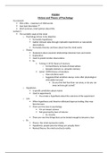
Summary lectures + reader Modelling Dynamic Systems
Lecture 1-3
System: single object or collection of interrelated objects that form a unified whole.
Systems -> separated from their environment/the surroundings by the system boundary
2 types of systems:
1. Closed system: system in which no information is exchanged with the surroundings.
2. Open system: system in which information is exchanged with the surroundings.
Model: simplified representation of a system.
Model has limited validity because of the simplifications.
Models in this course = mathematical representations of physical, chemical and biological systems
2 types of models:
1. Dynamic models: models which describe the change of a certain property over time and therefore
enable making predictions about the future development of that property.
2. Static models: models for static systems: systems in which we are not interested in the
dynamics/time-dependent behavior and only look to the steady state values because if changes
occur they are so fast (almost instant) that they are not relevant.
To distinguish dynamic models from static models you can look at the system equations -> a dynamic
𝑑…
model contains at least one equation with =
𝑑𝑡
𝑑…
= the state derivative/time derivative of the dynamic model
𝑑𝑡
Steady state value: value of a time-dependent variable when it doesn’t change in time anymore. ->
denote with subscript “ss” next to the symbol of the time-dependent variable
𝑑…
Steady state values are found by setting the state derivative of the dynamic model to zero -> =0
𝑑𝑡
Reasons to do modelling:
1. Models are useful when experiments are not possible, because experiments are:
- Too expensive
- Too dangerous
- Too slow (time scale of experiments is too big)
- Not possible because the system does not (yet) exist
2. Models are useful to:
- Improve understanding
- Design experiments
- Design controllers for systems
- Optimize systems
- Teach about the behavior of certain systems
Keywords of questions in modelling dynamic systems:
- “When”
- “How long”
- “How does it change”
,10 steps to create a mathematical model:
1. Make a sketch.
2. Draw the boundary of the system -> to distinguish what belongs to the system from what belongs
to the surroundings
3. Label the property which should be modelled.
4. Identify flow rates and fluxes that enter or leave the system.
5. Identify production or consumption rates of a property.
6. Write down the balance equation
7. Express all terms in mathematical expressions and simplify.
8. Check all units of the equations.
9. Define the initial conditions.
10. List all independent variables, dependent variables and model parameters.
General form of balance equation:
Change (accumulation) = flows in – flows out + production – consumption ± interfacial transfer
Balance equations usually rely on one of the following principles:
- Conservation of mass Balance equation always is one of the following:
- Conservation of energy - Mass balance
- Conservation of momentum - Energy balance
Different types of variables in models: - Force balance
1. Independent variables: variables which values are NOT dependent on any other variables (put on
x-axis in graph). -> in dynamic models independent variable is always time (t)!
2. Dependent variables: variables which values depend on the value of the independent variable (put
on y-axis in graph). -> in dynamic models these are all variables which change in time
3. Parameters: variables which are not independent variables nor dependent variables, because their
values don’t determine the values of the dependent variables and their values are not determined by
the value of the independent variable.
Coupled/complex mathematical models: mathematical models which consist of multiple (coupled)
balance equations instead of one single balance equation because there is a separate balance
equation needed for each dependent variable which should be modelled.
Creating coupled/complex mathematical models? -> use the 10 steps to create a mathematical
model, but make a separate balance equation for each dependent variable which should be
modelled
3 different types of mathematical models:
1. White box models: mathematical models which are derived purely from fundamental laws (e.g.
Newton’s laws).
2. Black box models: mathematical models which purely use empirical relations which don’t have
theoretical background but are solely determined by measurements.
3. Grey box models: mathematical models which use a combination of fundamental laws and
empirical relations.
Lecture 4
Variables in a mathematical model can be divided into 4 categories:
1. Inputs: variables that act from the environment onto the system.
- Controllable/manipulable inputs: inputs that you can choose.
- Disturbances: inputss which you cannot choose.
,2. Outputs: variables which you want to know and which are therefore measured -> often the state
variables, a combination of state variables or combinations of state and input variables
3. States: variables which describe the state/current situation in the system. -> all variables in
𝑑𝐶(𝑡)
derivatives except the time (t). e.g. -> C(t) = state
𝑑𝑡
4. Parameters: all remaining variables = constants.
States -> denoted with symbol x(t), so x1 = state variable 1, x2 = state variable 2 etc.
Inputs:
- Controllable/manipulable inputs -> denoted with symbol u(t), so u1 = input 1, u2 = input 2 etc.
- Disturbances -> denoted with symbol d(t)
Outputs -> denoted with symbol y(t), so y1 = output 1, y2 = output 2 etc.
Parameters -> denoted with symbol p, so p1 = parameter 1, p2 = parameter 2 etc.
Block diagram:
State-space mapping: using a state space map for writing down the balance equations of the model
using the symbols for states, inputs, outputs and parameters instead of the symbols of the quantities
so you can easily see if an equation is linear or non-linear.
State space map: table in which the quantities of the model are listed.
Symbol for type of variable Symbol quantity Description Units
x1 cx Biomass concentration kg m-3
u1 φv Volumetric flow rate m3 s-1
y1 cx Biomass concentration kg m-3
p1 V Volume m3
Linear equation -> NO multiplications of states or inputs
Non-linear equation -> multiplications of states or inputs
Essential questions in this course:
If we change the inputs of the system:
1. What is the end value?
2. How long does it take to reach the end value?
3. What happens in between?
Steady state value: value of a time-dependent variable when it doesn’t change in time anymore. ->
denote with subscript “ss” next to the symbol of the time-dependent variable
System is in steady state when all derivatives in the balance equations describing the system are
equal to zero!
, 2 ways for finding steady state values:
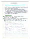
1. Analytically = set all state derivatives equal to zero:
Always write a-1 * b instead of a/b to prevent problems when a is a vector or matrix
2. Numerically = Newton-Raphson method: iterative search method for finding the solution of f(x) = 0
using the following formula:
Ways for denoting derivatives:
First derivative:
𝑑𝑥
= ẋ = x′(t)
𝑑𝑡
Lecture 1-3
System: single object or collection of interrelated objects that form a unified whole.
Systems -> separated from their environment/the surroundings by the system boundary
2 types of systems:
1. Closed system: system in which no information is exchanged with the surroundings.
2. Open system: system in which information is exchanged with the surroundings.
Model: simplified representation of a system.
Model has limited validity because of the simplifications.
Models in this course = mathematical representations of physical, chemical and biological systems
2 types of models:
1. Dynamic models: models which describe the change of a certain property over time and therefore
enable making predictions about the future development of that property.
2. Static models: models for static systems: systems in which we are not interested in the
dynamics/time-dependent behavior and only look to the steady state values because if changes
occur they are so fast (almost instant) that they are not relevant.
To distinguish dynamic models from static models you can look at the system equations -> a dynamic
𝑑…
model contains at least one equation with =
𝑑𝑡
𝑑…
= the state derivative/time derivative of the dynamic model
𝑑𝑡
Steady state value: value of a time-dependent variable when it doesn’t change in time anymore. ->
denote with subscript “ss” next to the symbol of the time-dependent variable
𝑑…
Steady state values are found by setting the state derivative of the dynamic model to zero -> =0
𝑑𝑡
Reasons to do modelling:
1. Models are useful when experiments are not possible, because experiments are:
- Too expensive
- Too dangerous
- Too slow (time scale of experiments is too big)
- Not possible because the system does not (yet) exist
2. Models are useful to:
- Improve understanding
- Design experiments
- Design controllers for systems
- Optimize systems
- Teach about the behavior of certain systems
Keywords of questions in modelling dynamic systems:
- “When”
- “How long”
- “How does it change”
,10 steps to create a mathematical model:
1. Make a sketch.
2. Draw the boundary of the system -> to distinguish what belongs to the system from what belongs
to the surroundings
3. Label the property which should be modelled.
4. Identify flow rates and fluxes that enter or leave the system.
5. Identify production or consumption rates of a property.
6. Write down the balance equation
7. Express all terms in mathematical expressions and simplify.
8. Check all units of the equations.
9. Define the initial conditions.
10. List all independent variables, dependent variables and model parameters.
General form of balance equation:
Change (accumulation) = flows in – flows out + production – consumption ± interfacial transfer
Balance equations usually rely on one of the following principles:
- Conservation of mass Balance equation always is one of the following:
- Conservation of energy - Mass balance
- Conservation of momentum - Energy balance
Different types of variables in models: - Force balance
1. Independent variables: variables which values are NOT dependent on any other variables (put on
x-axis in graph). -> in dynamic models independent variable is always time (t)!
2. Dependent variables: variables which values depend on the value of the independent variable (put
on y-axis in graph). -> in dynamic models these are all variables which change in time
3. Parameters: variables which are not independent variables nor dependent variables, because their
values don’t determine the values of the dependent variables and their values are not determined by
the value of the independent variable.
Coupled/complex mathematical models: mathematical models which consist of multiple (coupled)
balance equations instead of one single balance equation because there is a separate balance
equation needed for each dependent variable which should be modelled.
Creating coupled/complex mathematical models? -> use the 10 steps to create a mathematical
model, but make a separate balance equation for each dependent variable which should be
modelled
3 different types of mathematical models:
1. White box models: mathematical models which are derived purely from fundamental laws (e.g.
Newton’s laws).
2. Black box models: mathematical models which purely use empirical relations which don’t have
theoretical background but are solely determined by measurements.
3. Grey box models: mathematical models which use a combination of fundamental laws and
empirical relations.
Lecture 4
Variables in a mathematical model can be divided into 4 categories:
1. Inputs: variables that act from the environment onto the system.
- Controllable/manipulable inputs: inputs that you can choose.
- Disturbances: inputss which you cannot choose.
,2. Outputs: variables which you want to know and which are therefore measured -> often the state
variables, a combination of state variables or combinations of state and input variables
3. States: variables which describe the state/current situation in the system. -> all variables in
𝑑𝐶(𝑡)
derivatives except the time (t). e.g. -> C(t) = state
𝑑𝑡
4. Parameters: all remaining variables = constants.
States -> denoted with symbol x(t), so x1 = state variable 1, x2 = state variable 2 etc.
Inputs:
- Controllable/manipulable inputs -> denoted with symbol u(t), so u1 = input 1, u2 = input 2 etc.
- Disturbances -> denoted with symbol d(t)
Outputs -> denoted with symbol y(t), so y1 = output 1, y2 = output 2 etc.
Parameters -> denoted with symbol p, so p1 = parameter 1, p2 = parameter 2 etc.
Block diagram:
State-space mapping: using a state space map for writing down the balance equations of the model
using the symbols for states, inputs, outputs and parameters instead of the symbols of the quantities
so you can easily see if an equation is linear or non-linear.
State space map: table in which the quantities of the model are listed.
Symbol for type of variable Symbol quantity Description Units
x1 cx Biomass concentration kg m-3
u1 φv Volumetric flow rate m3 s-1
y1 cx Biomass concentration kg m-3
p1 V Volume m3
Linear equation -> NO multiplications of states or inputs
Non-linear equation -> multiplications of states or inputs
Essential questions in this course:
If we change the inputs of the system:
1. What is the end value?
2. How long does it take to reach the end value?
3. What happens in between?
Steady state value: value of a time-dependent variable when it doesn’t change in time anymore. ->
denote with subscript “ss” next to the symbol of the time-dependent variable
System is in steady state when all derivatives in the balance equations describing the system are
equal to zero!
, 2 ways for finding steady state values:
1. Analytically = set all state derivatives equal to zero:
Always write a-1 * b instead of a/b to prevent problems when a is a vector or matrix
2. Numerically = Newton-Raphson method: iterative search method for finding the solution of f(x) = 0
using the following formula:
Ways for denoting derivatives:
First derivative:
𝑑𝑥
= ẋ = x′(t)
𝑑𝑡