CS 234 ASSIGNMENT 2 2021/2022.
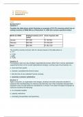
CS 234 ASSIGNMENT 2 2021/2022. Introduction In this assignment we will implement deep Q-learning, following DeepMind’s paper ([1] and [2]) that learns to play Atari games from raw pixels. The purpose is to demonstrate the effectiveness of deep neural networks as well as some of the techniques used in practice to stabilize training and achieve better performance. In the process, you’ll become familiar with PyTorch. We will train our networks on the Pong-v0 environment from OpenAI gym, but the code can easily be applied to any other environment. In Pong, one player scores if the ball passes by the other player.An episode is over when one of the players reaches 21 points. Thus, the total return of an episode is between −21 (lost every point) and +21 (won every point). Our agent plays against a decent hard-coded AI player. Average human performance is −3 (reported in [2]). In this assignment, you will train an AI agent with super-human performance, reaching at least +10 (hopefully more!). 1 CS 234 Winter 2021: Assignment #2 0 Distributions induced by a policy (13 pts) In this problem, we’ll work with an infinite-horizon MDP M = hS, A, R, T , γi and consider stochastic policies of the form π : S → ∆(A) 1 . Additionally, we’ll assume that M has a single, fixed starting state s 0 ∈ S for simplicity. (a) (written, 3 pts) Consider a fixed stochastic policy and imagine running several rollouts of this policy within the environment. Naturally, depending on the stochasticity of the MDP M and the policy itself, some trajectories are more likely than others. Write down an expression for ρ π (τ ), the likelihood of sampling a trajectory τ = (s 0 , a0 , s1 , a1, . . .) by running π in M. To put this distribution in context, recall that V π (s0) = E τ ρ ∼ π P∞ t=0 γ t R(s t , at) | s0 . Solution: ρ π (τ ) = ∞Y t=0 π(at |st)T (st+1 |st , at) (b) (written, 5 pts) Just as ρ π captures the distribution over trajectories induced by π, we can also examine the distribution over states induced by π. In particular, define the discounted, stationary state distribution of a policy π as d π (s) = (1 − γ) ∞X t=0 γ t p(st = s), where p(st = s) denotes the probability of being in state s at timestep t while following policy π; your answer to the previous part should help you reason about how you might compute this value. Consider an arbitrary function f : S × A → R. Prove the following identity: Eτ ρ ∼ π " ∞X t=0 γ t f (st , at) # = 1 (1 − γ) Es d ∼ π Ea π∼ (s) [f (s, a)] . Hint: You may find it helpful to first consider how things work out for f (s, a) = 1, ∀(s, a) S × A. ∈ Hint: What is p(s t = s)? Solution: Eτ ρ ∼ π " ∞X t=0 γ t f (st , at ) # = ∞X t=0 γ t Eτ ρ ∼ π [f (st , at)] = E τ ρ ∼ π [f (s0 , a0)] + γE τ ρ ∼ π [f (s1 , a1)] + γ 2Eτ ρ ∼ π [f (s2 , a2)] + ... = X a0 π(a0 |s0)f (s 0 , a0) + γ X a0 π(a0 |s0) X s1 T (s1 |s0 , a0) X a1 π(a1 |s1)f (s 1 , a1) + ... = X s p(s0 = s)E a π∼ (s) [f (s, a)] + γ X s p(s1 = s)E a π∼ (s) [f (s, a)] + ... = X s ∞X t=0 γ t p(st = s)E a π∼ (s) [f (s, a)] = 1 (1 − γ) X s d π (s)Ea π∼ (s) [f (s, a)] = 1 (1 − γ) Es d ∼ π Ea π∼ (s) [f (s, a)] 1For a finite set X , ∆(X ) refers to the set of categorical distributions with support on X or, equivalently, the ∆ |X |−1 probability simplex. Page 2 of 12 CS 234 Winter 2021: Assignment #2 (c) (written, 5 pts) For any policy π, we define the following function A π (s, a) = Q π (s, a) − V π (s). Prove the following statement holds for all policies π, π0 : V π (s0) − V π 0 (s0) = 1 (1 − γ) Es d ∼ π h Ea π∼ (s) h A π 0 (s, a) ii . Solution: V π (s0) − V π 0 (s0) = E τ ρ ∼ π " ∞X t=0 γ t R(s t , at) # − V π 0 (s0) = E τ ρ ∼ π " ∞X t=0 γ t R(s t , at) + V π 0 (st) − V π 0 (st) # − V π 0 (s0) = E τ ρ ∼ π " ∞X t=0 γ t R(s t , at) + γV π 0 (st+1 ) − V π 0 (st) # = E τ ρ ∼ π " E " ∞X t=0 γ t R(s t , at) + γV π 0 (st+1 ) − V π 0 (st ) st , at ## = E τ ρ ∼ π " ∞X t=0 γ t R(s t , at) + γE h V π 0 (st+1 ) st , at i − V π 0 (st) # = E τ ρ ∼ π " ∞X t=0 γ t Qπ 0 (st , at) − V π 0 (st) # = E τ ρ ∼ π " ∞X t=0 γ tA π 0 (st , at) # = 1 (1 − γ) Es d ∼ π h Ea π∼ (s) h A π 0 (s, a) ii . The function A π (s, a) is known as the advantage function which quantifies how much more advantageous it may (or may not) be to take action a in state s and follow policy π thereafter, rather than following policy π in state s. 1 Test Environment (6 pts) Before running our code on Pong, it is crucial to test our code on a test environment. In this problem, you will reason about optimality in the provided test environment by hand; later, to sanity-check your code, you will verify that your implementation is able to achieve this optimality. You should be able to run your models on CPU in no more than a few minutes on the following environment: • 4 states: 0, 1, 2, 3 • 5 actions: 0, 1, 2, 3, 4.Action 0 ≤ i ≤ 3 goes to state i, while action 4 makes the agent stay in the same state. • Rewards: Going to state i from states 0, 1, and 3 gives a reward R(i), where R(0) = 0.2, R(1) = −0.1, R(2) = 0.0, R(3) = −0.3. If we start in state 2, then the rewards defind above are multiplied by −10. See Table 1 for the full transition and reward structure. Page 3 of 12 CS 234 Winter 2021: Assignment #2 • One episode lasts 5 time steps (for a total of 5 actions) and always starts in state 0 (no rewards at the initial state). State (s) Action (a) Next State (s 0 ) Reward (R) 0 0 0 0.2 0 1 1 -0.1 0 2 2 0.0 0 3 3 -0.3 0 4 0 0.2 1 0 0 0.2 1 1 1 -0.1 1 2 2 0.0 1 3 3 -0.3 1 4 1 -0.1 2 0 0 -2.0 2 1 1 1.0 2 2 2 0.0 2 3 3 3.0 2 4 2 0.0 3 0 0 0.2 3 1 1 -0.1 3 2 2 0.0 3 3 3 -0.3 3 4 3 -0.3 Table 1: Transition table for the Test Environment An example of a trajectory (or episode) in the test environment is shown in Figure 5, and the trajectory can be represented in terms of st , at , Rt as: s0 = 0, a0 = 1, R0 = −0.1, s 1 = 1, a1 = 2, R1 = 0.0, s2 = 2, a2 = 4, R2 = 0.0, s3 = 2, a3 = 3, R3 = 3.0, s4 = 3, a4 = 0, R4 = 0.2, s5 = 0. Figure 1: Example of a trajectory in the Test Environment (a) (written 6 pts) What is the maximum sum of rewards that can be achieved in a single trajectory in the test environment, assuming γ = 1? Show first that this value is attainable in a single trajectory, and then briefly argue why no other trajectory can achieve greater cumulative reward. Solution: The optimal reward of the Test environment is Page 4 of 12 CS 234 Winter 2021: Assignment #2 6.2 To prove this, let’s prove an upper bound of 6.2 with 3 key observations • first, the maximum reward we can achieve is 3 when we do 2 → 3. • second, after having performed this optimal transition, we have to wait at least one step to execute it again. As we have 5 steps, we can execute 2 optimal moves. Executing less than 2 would yield a strictly smaller result. We need to go to 2 twice, which gives us 0 reward on 2 steps.Thus, we know that 4 steps gives us a max of 6. Then, the best reward we can achieve that is not an optimal move (starting from state 1) is 0.2, which yields an upper bound of 6.2. Considering the path 0 → 2 → 3 → 2 → 3 → 0 proves that we can achieve this upper bound.
Written for
- Institution
- Stanford University
- Course
- CS 234 (CS234)
Document information
- Uploaded on
- April 17, 2022
- Number of pages
- 13
- Written in
- 2021/2022
- Type
- Exam (elaborations)
- Contains
- Questions & answers
Subjects
-
cs 234
-
cs 234 assignment 2
-
cs 234 assignment
-
cs 234 assignment 2 20212022
-
cs 234 20212022
-
assignment 2 20212022

