Advanced statistics notes
Lecture 1
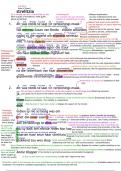
Assumptions linear regression
Homoskedasticity
,*violation that can only occur to time series data, so there needs to be some kind of order in the x-
variable. So when you have cross-sectional data (survey) you don’t have to worry about
autocorrelation, cause there is no natural order in the x-variable.
There should be a bell shaped distribution (but the assumption is not really that important)
,
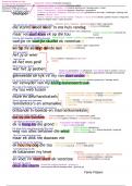
, Lecture 2: clustered data
Basic principles of mixed model analysis.
Back to the basics of linear regression. You have a scatterplot of all the observations, than you draw a
line through the dots and the characteristic of that line is that the distance from the line and the dots
is as least as possible (idea behind linear regression analysis). The regression line is the best way to
explain the linear relationship between y and x.
The line has 2 parameters, regression coefficients: b0 and b1.
- b0 is the value of the outcome when the independent variable(s) equals 0.
- b1 indicates how much the outcome differs with each unit difference from the independent
variable
If we want to correct for area, the b2 now means the difference in average health between area
number 1 and 2. But it is also an estimation of the difference in average health between area number
2 and 3, and area number 10 and 11. In other words: we assume a linear relationship between the
numbering of the area and the outcome variable health. That does not make any sense! You can’t do
this, area is not a continuous or discrete variable: it is a categorical varaible. Dummy’s in the
regression! 49 dummy variables for area, but not efficient to just adjust for area. You’re interested in
the relation between health and PA and you just want to adjust for area. and you’ll lose power..
Solution: using mixed model analysis. Efficient way to deal with a categorical variable with many
groups
In a mixed model there is a three steps method behind the scene:
1. estimate the intercepts for all groups
2. create a normal distribution over all the intercepts
3. estimate the variance of the normal distribution
Lecture 1
Assumptions linear regression
Homoskedasticity
,*violation that can only occur to time series data, so there needs to be some kind of order in the x-
variable. So when you have cross-sectional data (survey) you don’t have to worry about
autocorrelation, cause there is no natural order in the x-variable.
There should be a bell shaped distribution (but the assumption is not really that important)
,
, Lecture 2: clustered data
Basic principles of mixed model analysis.
Back to the basics of linear regression. You have a scatterplot of all the observations, than you draw a
line through the dots and the characteristic of that line is that the distance from the line and the dots
is as least as possible (idea behind linear regression analysis). The regression line is the best way to
explain the linear relationship between y and x.
The line has 2 parameters, regression coefficients: b0 and b1.
- b0 is the value of the outcome when the independent variable(s) equals 0.
- b1 indicates how much the outcome differs with each unit difference from the independent
variable
If we want to correct for area, the b2 now means the difference in average health between area
number 1 and 2. But it is also an estimation of the difference in average health between area number
2 and 3, and area number 10 and 11. In other words: we assume a linear relationship between the
numbering of the area and the outcome variable health. That does not make any sense! You can’t do
this, area is not a continuous or discrete variable: it is a categorical varaible. Dummy’s in the
regression! 49 dummy variables for area, but not efficient to just adjust for area. You’re interested in
the relation between health and PA and you just want to adjust for area. and you’ll lose power..
Solution: using mixed model analysis. Efficient way to deal with a categorical variable with many
groups
In a mixed model there is a three steps method behind the scene:
1. estimate the intercepts for all groups
2. create a normal distribution over all the intercepts
3. estimate the variance of the normal distribution