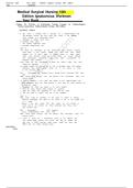
• It is the local trade off between w and R relevant to the marginal firm and
marginal worker at a given risk
• The slope of the HWF measures the cost and benefit or risk reduction.
Only works for small changes
• In diagram, we consider when risk falls from R1 to R2. This is a large
change.
• The HWF underestimates this at Δw
• We consider 2 different types of workers. If the librarian wants to be a test
pilot, she will incur risk RT so she be given wage wL’. To be a librarian, the
test pilot needs a higher wage than the librarians current one of wL
Testing the compensating differentials hypothesis
• i= individuals, X=personal characteristics, J= job characteristics
• J can be measured by workers’ self-reported responses or objective data
at a level of industry or occupation.
• Means all individuals in the industry are assigned the same characteristics.
• Let j=1 be most pleasant job, j=2 be less present etc. Then we expect that γ<0
• Evidence is inconclusive- gamma is statistically insignificant or of the wrong sign
• May be due to no compensating differentials due to labour market imperfections which prevent
flows or due to econometric issues.
• Gamma may be biased due to measurement error and omitted variable bias.
• To solve, we use longitudinal data to eliminate fixed effects and use instrumental variables.
• We consider where employers pay for the health insurance offered to workers or whether they
reduce wages to offset the costs. If this is true workers will match themselves with firms offering
insurance and paying lower wages.
• There will be a compensating differential – wages lower when there is EPHI, ceteris paribus.
• Olson (2002) estimated ln Wi=α0+ α1Di+α2Xi+ei . D is dummy, equals 1 if receives insurance
• We expect α1 to be negative. Olsen found that full-time working women receiving EPHI accept a
wage lower (by between 10 and 23%) than the wage paid in the absence of EPHI.
Value of Life
• We consider annual fatality rates per 100,000 employees. In manufacturing, this rate is 0.00004
whilst in construction it is 0.00024. Assume that a worker in construction earns £600 more, per
annum, than a worker in manufacturing.
• Differential is 0.0002
• Value of life= dw/dR= differential wage/differential risk= 600/0.0002=£3million
• N.b only a statistical figure and shouldn’t be used to determine compensation. Used when
deciding to build safer motorway
Misperceptions of Risk
• Many people underestimate larger risks
• E.g. assume the wage rises. Individuals believe the change in risk is ΔRp but
in reality it is much larger at ΔRA
• This can justify gov intervention. We assume asymmetric info- only firms
know true risk
• The individual believes that they are at point B on the dotted IC.
• However, in reality they are at point A with a much higher risk.
• The gov imposes a max risk level below that prevailing in risky jobs- sets RMax
• We end up at point C. Firms are on their same isoprofit so are no worse off.
• Workers are better off in reality- on a higher IC at C than A so higher utility
- However, their perceived utility falls
, Compensating Wage Differentials
• As long as workers or firms can freely enter and exit a competitive labor market, there will be a
single wage in the economy if all jobs are alike and all workers are alike.
• We now drop the assumption of homogenous workers and jobs
• Wage differentials are the means by which labour market achieves matching and the result of
the matching process
• Heterogeneity: differences between workers- gender, preferences and skills.
- Non pecuniary differences between jobs- risk , job security, pleasantness
• With heterogeneity, we get wage differentials. The utility of the overall compensation package is
equalised
- i.e. utility of the wage plus utility of non-pecuniary job characteristics
• There are two jobs, 1 and 2, with wages w1 and w2 and non-wage characteristics J1 and J2.
• An individual will be indifferent between the two jobs when U(w1, J1)=U(w2, J2)
- The equilibrium arises as workers ‘pay’ for desirable job characteristics by accepting lower
wages. So, an unpleasant job will pay more.
• Assumptions: workers max utility, workers well informed about job characteristics and workers
have the choice and mobility to move between jobs.
• E.g. all workers have preferences shown by U= w - 2x where w is the wage.
• There are two types of jobs: clean job x=0 and dirty job x=1. Clean job plays $16 an hour
• At equilibrium Udirty=Uclean w - 2(1) = w - 2(0) . We get w0=$36 so differential is $20
Model
• Assume only non-wage characteristic is risk (accident/death) and that
individuals are risk averse
• Diagram shows IC of individuals. Slopes rises as we go along IC as disutility of
risk increases
•Dotted line is for someone who is less risk averse
•The employer: assume it is costly to reduce risk and perfect
competition
•When the firm reduces risk, it incurs costs so it must reduce
wages to remain competitive.
•We plot isoprofits. The higher the isoprofit, the lower the
profit
•Dashed isoprofit: less costly to reduce risk
•We see that type A individuals, who are risk averse, match
themselves with type a firms, who find it cheaper to reduce risk
•On the offer curve, those combos will not be chosen
Hedonic wage function
• Function shows many different types of firms and customers hence
different ICs and isoprofits
• Gives the wage-risk combinations that will be observed in the labor
market
• Provided individuals are risk-averse, more risky jobs will pay a wage
premium, a compensating differential.
• Firms and workers match in a non-random way. Safe firms are matched with safety-loving
workers .
- The more risk-averse individuals take jobs in firms which can reduce risk more cheaply.
• The slope of the hedonic wage function represents the marginal supply and demand price of
risk
- Since at tangency, MCrisk reduction = MBrisk reduction
, Labour Demand
• The firm’s production function is q=f(L,K), describes the tech that the firm uses to produce
output. L is number of employee hours .
• MPL is the marginal product of labour
• marginal curve lies below the average curve when the average curve is falling.
• Profits = pq - wL - rK . r is capital price, w is wage rate
employment decision in short run
• in short run, capital is fixed. MRP=MP x P
• A profit-maximising firm hires workers up to the point where the wage rate equals the value of
marginal product of labor.
• e.g. extra worker makes £10 of output and wage is £8 so hires worker. We assume firm cannot
influence the wage- it’s taken as given
• short run demand curve shifts up when productivity rises or
price of output rises
• short run elasticity of demand:
The Employment Decision in the Long Run
• Capital stock is not fixed. Isoquant gives labour and capital combos that give same output. The
slope of the isoquant is -MPL/MPK. Absolute value of this is MRTS and it’s diminishing
• C=wl+rK, isocost gives combos that gives one cost. Rearrange, K= C/r - w/r L . This is of form
y=mx+c and so slope is -w/r
• cost min occurs at tangency, when MPL/MPK = w/r (slope of isoquant equals slope of isocost)
or MRTS= ratio of input prices
• a profit-maximising firm hires each input up to the point where the price of the input equals the
value of marginal product of the input. This implies that the optimal input mix is where the ratio
of marginal products of labor and capital equals the ratio of input prices.
• Long run profit max requires w=pMPL and r=pMPK. These profit max conditions
imply cost minimisation
• The Long-Run Demand Curve for Labor
• We consider what happens when the wage changes. Firm initially produces q0,
the profit max level of output. It wants to do this at the lowest cost so does ratio
of MP= ratio of input prices
• Wage was w0 and it falls to w1. isocost is flatter. Note there’s a new intercept for
the isocost- it is now the TC for making 150 units
• a wage cut always increases the amount of workers hired but may increase or
decrease capital
• We decompose a wage change into substitution and scale effects for hiring
• wage cut reduces the price of labor relative to capital. The fall in the wage
encourages the firm to readjust its input mix to make it labor intensive
• In addition, the wage cut reduces the marginal cost of production and
encourages the firm to expand. As the firm expands, it wants to hire even
more workers.
• The firm begins at P. The wage falls. Plot a new isocost, parallel to original.
• so the firm takes advantage of the lower price of labour by expanding
production (move from P to Q). The scale effect indicates what happens to
the demand for the firm’s inputs as the firm expands production.
• The firm then takes advantage of the wage change by rearranging its mix of
inputs ( switch from capital to labour) whilst holding output constant. This is
the substitution effect from Q to R. The sub effect must decrease the firm’s
demand for capital. Here, the scale dominates sub effect so capital and labour rise
• Long run labour demand curve is more elastic than short run demand curve as capital can also
be adjusted so firm can adjust its size easily
• Empirical suggests short run labour demand elasticity lies between 0.4 and 0.5. a 10% increase
in the wage reduces employment by 4 to 5 percentage points in the short run