FINM6222 LU3 – Cost-Volume-Profit
Analysis
3.1 Intro
CVP analyses the effect on profit & costs to changes in:
- Variable costs
- Fixed costs
- Selling prices
- Volume
- Product mix
CVP analysis enables management to plan and cope w planning decisions
3.2 Underlying assumptions
- costs and revenues exhibit a linear behavior throughout a given activity range
- costs can be accurately classified as either fixed or variable
- costs are affected by changes in activity levels only
- there is a short-term planning period
- all units produced are sold
- when a company sells more than one product type, the sales mix remains constant.
3.3 CVP Graphs
3.3.1 Economist CVP Graph
The total revenue line is curvi-linear bc a business can only sell
more units if it drops it selling price per unit. At first, revenue grows,
but later it slows down and can even fall if prices get too low.
Cost Curve Stages:
A-B: Costs shoot up quickly at low output. This happens because
the company is running below the facility’s efficient scale, the plant
is built for higher volumes, so operating at small levels is inefficient
(decreasing returns to scale).
B-C: Costs rise more slowly as production increases. At this point, the factory is running
efficiently, benefiting from specialisation and better production schedules (increasing returns
to scale).
C-D: Costs start climbing faster again as production gets pushed too high. Complexity,
bottlenecks, and overcapacity make operations less efficient.
B and C are the break-even points – profit is at a max where the distance btwn the cost and
revenue lines is the largest.
, 3.3.2 Accountant CVP Graph
The accountant’s CVP graph uses the variable costing method.
This means the selling price per unit and variable cost per unit are
assumed to stay the same which creates linear revenue and cost
lines. There is only one break-even point (where revenue = costs).
Profit increases steadily as more units are sold, and the profit area
gets wider with higher sales. Fixed costs stay constant no matter
how many units are produced, so they’re shown as a flat horizontal
line.
3.3.3 Economists vs Accountant View
Economist Accountant
Views a whole range of activity. Views only a relevant range over a short
period of time.
Assumes information on price, cost and Assumes limited availability price, cost and
volume is available at all levels of activity. volume info and linearity over a relevant
range.
View is expositional. View is practical
Two break-even points. Only 1 break-even point
3.4 CVP Analysis – A Mathematical Approach
3.4.1 Basic Equations
Net profit is represented by: NP = Px – (a + bx)
x = units sold
P = selling price
b = variable cost per unit
a = total fixed cost
3.4.2 Break-even analysis
This determines the break-even point, determined in 2 ways:
- Break-even sales (units) = fixed costs / unit contribution margin
- Break-even sales (rands) = fixed costs / unit contribution ratio
OR break-even sales (units) x selling price per unit
Analysis
3.1 Intro
CVP analyses the effect on profit & costs to changes in:
- Variable costs
- Fixed costs
- Selling prices
- Volume
- Product mix
CVP analysis enables management to plan and cope w planning decisions
3.2 Underlying assumptions
- costs and revenues exhibit a linear behavior throughout a given activity range
- costs can be accurately classified as either fixed or variable
- costs are affected by changes in activity levels only
- there is a short-term planning period
- all units produced are sold
- when a company sells more than one product type, the sales mix remains constant.
3.3 CVP Graphs
3.3.1 Economist CVP Graph
The total revenue line is curvi-linear bc a business can only sell
more units if it drops it selling price per unit. At first, revenue grows,
but later it slows down and can even fall if prices get too low.
Cost Curve Stages:
A-B: Costs shoot up quickly at low output. This happens because
the company is running below the facility’s efficient scale, the plant
is built for higher volumes, so operating at small levels is inefficient
(decreasing returns to scale).
B-C: Costs rise more slowly as production increases. At this point, the factory is running
efficiently, benefiting from specialisation and better production schedules (increasing returns
to scale).
C-D: Costs start climbing faster again as production gets pushed too high. Complexity,
bottlenecks, and overcapacity make operations less efficient.
B and C are the break-even points – profit is at a max where the distance btwn the cost and
revenue lines is the largest.
, 3.3.2 Accountant CVP Graph
The accountant’s CVP graph uses the variable costing method.
This means the selling price per unit and variable cost per unit are
assumed to stay the same which creates linear revenue and cost
lines. There is only one break-even point (where revenue = costs).
Profit increases steadily as more units are sold, and the profit area
gets wider with higher sales. Fixed costs stay constant no matter
how many units are produced, so they’re shown as a flat horizontal
line.
3.3.3 Economists vs Accountant View
Economist Accountant
Views a whole range of activity. Views only a relevant range over a short
period of time.
Assumes information on price, cost and Assumes limited availability price, cost and
volume is available at all levels of activity. volume info and linearity over a relevant
range.
View is expositional. View is practical
Two break-even points. Only 1 break-even point
3.4 CVP Analysis – A Mathematical Approach
3.4.1 Basic Equations
Net profit is represented by: NP = Px – (a + bx)
x = units sold
P = selling price
b = variable cost per unit
a = total fixed cost
3.4.2 Break-even analysis
This determines the break-even point, determined in 2 ways:
- Break-even sales (units) = fixed costs / unit contribution margin
- Break-even sales (rands) = fixed costs / unit contribution ratio
OR break-even sales (units) x selling price per unit