Deep Learning – Lecture 1
History
● Perceptron: Frank Rosenbladt was the first to invent the Perceptron
● Back propagation: Several researchers in the 1980’s
● Big Data:
o Andrew Ng (Cat experiment)
o Fei-Fei Li (ImageNet) An image database organized according to the WordNet
hierarchy. Each node in this hierarchy represented thousands of images.
o AlexNet 🡪 Deep CNN trained on ImageNet using GPU’s
Practical Deep Learning
Although most computers (like your laptop) have a CPU (Central Processing Unit) this is not optimal
for running Deep Neural Networks. Despite the fact that it can handle a diverse workload, the
computation is done in a serial manner. This way of computation will result in very slow training.
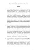
A better approach is the use of a GPU (Graphical Processing Unit) which can only handle a specific
workload, but computes this in a parallel fashion which is much more efficient, especially since the
computations in a neural network are easy to break down in similar smaller computations. The
difference is clearly illustrated in this video. An explanation can be found here.
Deep learning environments
,Perceptron
- Most basic single-layer NN
⇒ typically used for binary classification problems (1 or 0, “yes” or “no”)
- Data needs to be linearly separable (if the decision boundary is non-linear, the
perceptron can’t be used).
- Goal: find a line that splits the data/observations
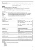
How does a perceptron work?
Our inputs (Xi) are each multiplied by weights (Wi). The outputs are combined in a summed
input function that is passed on to an activation function (Step function). The activation
function determines if the network classifies the input (y’) as 1 or 0 based on a threshold (t)
,NOTE: one f the inputs is the bias. Without the bias, the function has to go through the
origin, and that is not always what we want!
Activation function
● the output node has a threshold t
○ if summed input ≥ t, then it ‘fires’ (output y’=1)
○ if summed input < t, then it doesn’t ‘fire’ (output y’=0
● We can rewrite the activation function. t is moved to the other side of the equation
creating a situation where:
○ 0 or higher = 1
○ Lower than 0 = 0
NOTE: Eva: Threshold = bias
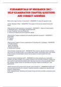
Update rule
How can the perceptron now learn a good set of weights/bias? If the expected output is not
equal to the observed output (i.e. y’ ≠ y) the weights (and bias) need to be updated
accordingly:
If y’ is not equal to y, then the learning rate
and xi will be multiplied by either -1 or 1.
→ as this resulting value is added to wi, the
weight will bet smaller/larger
→ e.g. wi + 0.1 * xi * (-1) < wi
, If y and y’ are equal, the learning rate and xi will be multiplied by 0.
→ wi + 0 = wi → therefore the weights won’t change if the prediction was correct.
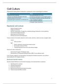
AND Gate
AND gate fire 1 ONLY when both inputs are 1.
In the example below we can see how the w&b are adjusted as we train. In this example, X3
is the bias and W3 is the weight that corresponds to the bias. We have a learning rate of 1.
● We see that the first example yields: y’= 1
while y = 0
→ this leads to an update rule:
○ w1_new = 0.5 + 1 * 0 * (-1) = 0.5
○ w2_new = 0.5 + 1 * 0 * (-1) = 0.5
○ W3_new = 0 + 1 * 1 * (-1) = -1
● The second row yields: y’ = 0 and y = 0
because:
0 * 0.5 + 1 * 0.5 + 1 * -1 = -0.5
→ because -0.5 < 0 we predict 0
→ we do not update the weights because the prediction is correct
● The same accounts for the third and fourth prediction
History
● Perceptron: Frank Rosenbladt was the first to invent the Perceptron
● Back propagation: Several researchers in the 1980’s
● Big Data:
o Andrew Ng (Cat experiment)
o Fei-Fei Li (ImageNet) An image database organized according to the WordNet
hierarchy. Each node in this hierarchy represented thousands of images.
o AlexNet 🡪 Deep CNN trained on ImageNet using GPU’s
Practical Deep Learning
Although most computers (like your laptop) have a CPU (Central Processing Unit) this is not optimal
for running Deep Neural Networks. Despite the fact that it can handle a diverse workload, the
computation is done in a serial manner. This way of computation will result in very slow training.
A better approach is the use of a GPU (Graphical Processing Unit) which can only handle a specific
workload, but computes this in a parallel fashion which is much more efficient, especially since the
computations in a neural network are easy to break down in similar smaller computations. The
difference is clearly illustrated in this video. An explanation can be found here.
Deep learning environments
,Perceptron
- Most basic single-layer NN
⇒ typically used for binary classification problems (1 or 0, “yes” or “no”)
- Data needs to be linearly separable (if the decision boundary is non-linear, the
perceptron can’t be used).
- Goal: find a line that splits the data/observations
How does a perceptron work?
Our inputs (Xi) are each multiplied by weights (Wi). The outputs are combined in a summed
input function that is passed on to an activation function (Step function). The activation
function determines if the network classifies the input (y’) as 1 or 0 based on a threshold (t)
,NOTE: one f the inputs is the bias. Without the bias, the function has to go through the
origin, and that is not always what we want!
Activation function
● the output node has a threshold t
○ if summed input ≥ t, then it ‘fires’ (output y’=1)
○ if summed input < t, then it doesn’t ‘fire’ (output y’=0
● We can rewrite the activation function. t is moved to the other side of the equation
creating a situation where:
○ 0 or higher = 1
○ Lower than 0 = 0
NOTE: Eva: Threshold = bias
Update rule
How can the perceptron now learn a good set of weights/bias? If the expected output is not
equal to the observed output (i.e. y’ ≠ y) the weights (and bias) need to be updated
accordingly:
If y’ is not equal to y, then the learning rate
and xi will be multiplied by either -1 or 1.
→ as this resulting value is added to wi, the
weight will bet smaller/larger
→ e.g. wi + 0.1 * xi * (-1) < wi
, If y and y’ are equal, the learning rate and xi will be multiplied by 0.
→ wi + 0 = wi → therefore the weights won’t change if the prediction was correct.
AND Gate
AND gate fire 1 ONLY when both inputs are 1.
In the example below we can see how the w&b are adjusted as we train. In this example, X3
is the bias and W3 is the weight that corresponds to the bias. We have a learning rate of 1.
● We see that the first example yields: y’= 1
while y = 0
→ this leads to an update rule:
○ w1_new = 0.5 + 1 * 0 * (-1) = 0.5
○ w2_new = 0.5 + 1 * 0 * (-1) = 0.5
○ W3_new = 0 + 1 * 1 * (-1) = -1
● The second row yields: y’ = 0 and y = 0
because:
0 * 0.5 + 1 * 0.5 + 1 * -1 = -0.5
→ because -0.5 < 0 we predict 0
→ we do not update the weights because the prediction is correct
● The same accounts for the third and fourth prediction