ALL 11 CHAPTERS COVERED
SOLUTIONS MANUAL
,TABLE OF CONTENTS
Chapter 1 Introduction
Chapter 2 Pressure Distribution in a Fluid
Chapter 3 Integral Relations for a Control Volume
Chapter 4 Differential Relations for Fluid Flow
Chapter 5 Dimensional Analysis and Similarity
Chapter 6 Viscous Flow in Ducts
Chapter 7 Flow Past Immersed Bodies
Chapter 8 Potential Flow and Computational Fluid Dynamics
Chapter 9 Compressible Flow
Chapter 10 Open-Channel Flow
Chapter 11 Turbomachinery
APPENDIX F
, Chapter 1 Introduction 1-1
Chapter 1 Introduction
P1.1 A gas at 20C may be rarefied if it contains less than 1012 molecules per mm3. If
Avogadro’s number is 6.023E23 molecules per mole, what air pressure does this represent?
Solution: The mass of one molecule of air may be computed as
Molecular weight 28.97 mol 1
m 4.81E23 g
Avogadro’s number 6.023E23 molecules/g mol
Then the density of air containing 1012 molecules per mm3 is, in SI units,
molecules g
1012 3 4.81E23
mm molecule
g kg
4.81E11 3
4.81E5 3
mm m
Finally, from the perfect gas law, Eq. (1.13), at 20C 293 K, we obtain the pressure:
kg m2
p RT 4.81E5 3 287 2 (293 K) 4.0Pa ns.
m s K
Copyright © McGraw-Hill Education. All rights reserved. No reproduction or distribution without the prior written consent of
McGraw-Hill Education.
, Chapter 1 Introduction 1-2
P1.2 Table A.6 lists the density of the standard atmosphere as a function of altitude. Use
these values to estimate, crudely, say, within a factor of 2, the number of molecules of air in
the entire atmosphere of the earth.
Solution: Make a plot of density versus altitude z in the atmosphere, from Table A.6:
1.2255 kg/m3
Density in the Atmosphere
0 z 30,000 m
This writer’s approximation: The curve is approximately an exponential, o exp(-bz), with
b approximately equal to 0.00011 per meter. Integrate this over the entire atmosphere, with the
radius of the earth equal to 6377 km:
b z
d (vol ) 0 [ o e
2
matmosphere ](4 Rearth dz )
2
o 4 Rearth (1.2255 kg / m3 )4 (6.377 E 6 m)2
5.7 E18 kg
b 0.00011 / m
Dividing by the mass of one molecule 4.8E23 g (see Prob. 1.1 above), we obtain
the total number of molecules in the earth’s atmosphere:
m(atmosphere) 5.7E21 grams
N molecules 1.2Ε44 molecules Ans.
m(one molecule) 4.8E 23 gm/molecule
This estimate, though crude, is within 10 per cent of the exact mass of the atmosphere.
Copyright © McGraw-Hill Education. All rights reserved. No reproduction or distribution without the prior written consent of
McGraw-Hill Education.
, Chapter 1 Introduction 1-3
P1.3 For the triangular element in Fig.
P1.3, show that a tilted free liquid surface,
in contact with an atmosphere at pressure
pa, must undergo shear stress and hence
begin to flow.
Fig. P1.3
Solution: Assume zero shear. Due to
element weight, the pressure along the lower
and right sides must vary linearly as shown,
to a higher value at point C. Vertical forces
are presumably in balance with ele-ment
weight included. But horizontal forces are
out of balance, with the unbalanced force
being to the left, due to the shaded excess-
pressure triangle on the right side BC. Thus
hydrostatic pressures cannot keep the
element in balance, and shear and flow result.
P1.4 Sand, and other granular materials, definitely flow, that is, you can pour them
from a container or a hopper. There are whole textbooks on the “transport” of granular
materials [54]. Therefore, is sand a fluid? Explain.
Solution: Granular materials do indeed flow, at a rate that can be measured by
“flowmeters”. But they are not true fluids, because they can support a small shear stress
without flowing. They may rest at a finite angle without flowing, which is not possible for
liquids (see Prob. P1.3). The maximum such angle, above which sand begins to flow, is
called the angle of repose. A familiar example is sugar, which pours easily but forms a
significant angle of repose on a heaping spoonful. The physics of granular materials are
complicated by effects such as particle cohesion, clumping, vibration, and size
segregation. See Ref. 48 to learn more.
________________________________________________________________________
Copyright © McGraw-Hill Education. All rights reserved. No reproduction or distribution without the prior written consent of
McGraw-Hill Education.
, Chapter 1 Introduction 1-4
P1.5 A formula for estimating the mean free path of a perfect gas is:
ℓ 1.26 1.26 RT (1)
RT p
where the latter form follows from the ideal-gas law, pRT. What are the dimensions
of the constant “1.26”? Estimate the mean free path of air at 20C and 7 kPa. Is air rarefied
at this condition?
Solution: We know the dimensions of every term except “1.26”:
M M L2
{ℓ} {L} {} {} 3 {R} 2 {T} {}
LT L T
Therefore the above formula (first form) may be written dimensionally as
{M/LT}
{L} {1.26?} {1.26?}{L}
{M/L } [{L2 /T 2 }{}]
3
Since we have {L} on both sides, {1.26} {unity}, that is, the constant is dimensionless.
The formula is therefore dimensionally homogeneous and should hold for any unit system.
For air at 20C 293 K and 7000 Pa, the density is pRT (7000)/[(287)(293)] 0.0832
kgm3. From Table A-2, its viscosity is 1.80E5 N s/m2. Then the formula predicts
a mean free path of
1.80E5
ℓ 1.26 9.4E7 m Ans.
(0.0832)[(287)(293)]1/2
This is quite small. We would judge this gas to approximate a continuum if the physical
scales in the flow are greater than about 100 ℓ, that is, greater than about 94 m.
Copyright © McGraw-Hill Education. All rights reserved. No reproduction or distribution without the prior written consent of
McGraw-Hill Education.
, Chapter 1 Introduction 1-5
P1.6 Henri Darcy, a French engineer, proposed that the pressure drop Δp for flow at
velocity V through a tube of length L could be correlated in the form
p
LV 2
If Darcy’s formulation is consistent, what are the dimensions of the coefficient α?
Solution: From Table 1.2, introduce the dimensions of each variable:
p ML1T 2 L2 L2
ML
3 2 LV
2
L 2
T T
Solve for {α} = {L-1} Ans.
[The complete Darcy correlation is α = f /(2D), where D is the tube diameter, and f is a
dimensionless friction factor (Chap. 6).]
________________________________________________________________________
P1.7 Convert the following inappropriate quantities into SI units: (a) 2.283E7
U.S. gallons per day; (b) 4.48 furlongs per minute (racehorse speed); and (c)
72,800 avoirdupois ounces per acre.
Solution: (a) (2.283E7 gal/day) x (0.0037854 m3/gal) ÷ (86,400 s/day) =
1.0 m3/s Ans.(a)
(b) 1 furlong = (⅛)mile = 660 ft.
Then (4.48 furlongs/min)x(660 ft/furlong)x(0.3048 m/ft)÷(60 s/min) =
15 m/s Ans.(b)
(c) (72,800 oz/acre)÷(16 oz/lbf)x(4.4482 N/lbf)÷(4046.9 acre/m2) =
5.0 N/m2 = 5.0 Pa Ans.(c)
________________________________________________________________________
Copyright © McGraw-Hill Education. All rights reserved. No reproduction or distribution without the prior written consent of
McGraw-Hill Education.
, Chapter 1 Introduction 1-6
P1.8 Suppose that bending stress in a beam depends upon bending moment M and
beam area moment of inertia I and is proportional to the beam half-thickness y. Suppose
also that, for the particular case M 2900 inlbf, y 1.5 in, and I 0.4 in4, the predicted
stress is 75 MPa. Find the only possible dimensionally homogeneous formula for .
Solution: We are given that y fcn(M,I) and we are not to study up on strength of
materials but only to use dimensional reasoning. For homogeneity, the right hand side
must have dimensions of stress, that is,
M
{ } {y}{fcn(M,I)}, or: 2 {L}{fcn(M,I)}
LT
M
or: the function must have dimensions {fcn(M,I)} 2 2
L T
Therefore, to achieve dimensional homogeneity, we somehow must combine bending
moment, whose dimensions are {ML2T –2}, with area moment of inertia, {I} {L4}, and
end up with {ML–2T –2}. Well, it is clear that {I} contains neither mass {M} nor time {T}
dimensions, but the bending moment contains both mass and time and in exactly the com-
bination we need, {MT –2}. Thus it must be that is proportional to M also. Now we have
reduced the problem to:
M ML2 4
yM fcn(I), or 2
{L} 2 {fcn(I)}, or: {fcn(I)} {L }
LT T
We need just enough I’s to give dimensions of {L–4}: we need the formula to be exactly
inverse in I. The correct dimensionally homogeneous beam bending formula is thus:
My
C , where {C} {unity} Ans.
I
The formula admits to an arbitrary dimensionless constant C whose value can only be
obtained from known data. Convert stress into English units: (75 MPa)(6894.8)
10880 lbfin2. Substitute the given data into the proposed formula:
lbf My (2900 lbf in)(1.5 in)
10880 2
C C , or: C 1.00 Ans.
in I 0.4 in 4
The data show that C 1, or My/I, our old friend from strength of materials.
Copyright © McGraw-Hill Education. All rights reserved. No reproduction or distribution without the prior written consent of
McGraw-Hill Education.
, Chapter 1 Introduction 1-7
P1.9 A hemispherical container, 26 inches in diameter, is filled with a liquid at 20C
and weighed. The liquid weight is found to be 1617 ounces. (a) What is the density of
the fluid, in kg/m3? (b) What fluid might this be? Assume standard gravity, g = 9.807
m/s2.
Solution: First find the volume of the liquid in m3:
1 3 1 3 in 3
Hemisphere volume D 26 in 4601 in 61024 3 0.0754m 3
3
2 6 2 6 m
kg
Liquid mass 1617 oz 16 101 lbm 0.45359 45.84 kg
lbm
45.84 kg kg
Then the liquid density 3 607 3 Ans.(a)
0.0754 m m
From Appendix Table A.3, this could very well be ammonia. Ans.(b)
_______________________________________________________________________
P1.10 The Stokes-Oseen formula [10] for drag on a sphere at low velocity V is:
9
F 3 DV V2 D2
16
where D sphere diameter, viscosity, and density. Is the formula homogeneous?
Solution: Write this formula in dimensional form, using Table 1-2:
9
{F} {3 }{}{D}{V} {}{V}2 {D}2 ?
16
M L 2
2
ML M L
or: 2 {1} {L} {1} 3 2 {L } ?
T LT T L T
where, hoping for homogeneity, we have assumed that all constants (3,,9,16) are pure,
i.e., {unity}. Well, yes indeed, all terms have dimensions {MLT2}! Therefore the Stokes-
Oseen formula (derived in fact from a theory) is dimensionally homogeneous.
Copyright © McGraw-Hill Education. All rights reserved. No reproduction or distribution without the prior written consent of
McGraw-Hill Education.
, Chapter 1 Introduction 1-8
P1.11 In English Engineering units, the specific heat cp of air at room temperature is
approximately 0.24 Btu/(lbm-F). When working with kinetic energy relations, it is more
appropriate to express cp as a velocity-squared per absolute degree. Give the numerical
value, in this form, of cp for air in (a) SI units, and (b) BG units.
Solution: From Appendix C, Conversion Factors, 1 Btu = 1055.056 J (or N-m) = 778.17
ft-lbf, and 1 lbm = 0.4536 kg = (1/32.174) slug. Thus the conversions are:
_______________________________________________________________________
P1.12 For low-speed (laminar) flow in a tube of radius ro, the velocity u takes the form
p
uB
r 2
o r2
where is viscosity and p the pressure drop. What are the dimensions of B?
Solution: Using Table 1-2, write this equation in dimensional form:
{p} 2 L {M/LT 2} 2 L2
{u} {B} {r }, or: {B?} {L } {B?} ,
{} T {M/LT} T
or: {B} {L–1} Ans.
The parameter B must have dimensions of inverse length. In fact, B is not a constant, it
hides one of the variables in pipe flow. The proper form of the pipe flow relation is
p 2 2
uC
L
ro r
where L is the length of the pipe and C is a dimensionless constant which has the theoretical
laminar-flow value of (1/4)—see Sect. 6.4.
Copyright © McGraw-Hill Education. All rights reserved. No reproduction or distribution without the prior written consent of
McGraw-Hill Education.
SOLUTIONS MANUAL
,TABLE OF CONTENTS
Chapter 1 Introduction
Chapter 2 Pressure Distribution in a Fluid
Chapter 3 Integral Relations for a Control Volume
Chapter 4 Differential Relations for Fluid Flow
Chapter 5 Dimensional Analysis and Similarity
Chapter 6 Viscous Flow in Ducts
Chapter 7 Flow Past Immersed Bodies
Chapter 8 Potential Flow and Computational Fluid Dynamics
Chapter 9 Compressible Flow
Chapter 10 Open-Channel Flow
Chapter 11 Turbomachinery
APPENDIX F
, Chapter 1 Introduction 1-1
Chapter 1 Introduction
P1.1 A gas at 20C may be rarefied if it contains less than 1012 molecules per mm3. If
Avogadro’s number is 6.023E23 molecules per mole, what air pressure does this represent?
Solution: The mass of one molecule of air may be computed as
Molecular weight 28.97 mol 1
m 4.81E23 g
Avogadro’s number 6.023E23 molecules/g mol
Then the density of air containing 1012 molecules per mm3 is, in SI units,
molecules g
1012 3 4.81E23
mm molecule
g kg
4.81E11 3
4.81E5 3
mm m
Finally, from the perfect gas law, Eq. (1.13), at 20C 293 K, we obtain the pressure:
kg m2
p RT 4.81E5 3 287 2 (293 K) 4.0Pa ns.
m s K
Copyright © McGraw-Hill Education. All rights reserved. No reproduction or distribution without the prior written consent of
McGraw-Hill Education.
, Chapter 1 Introduction 1-2
P1.2 Table A.6 lists the density of the standard atmosphere as a function of altitude. Use
these values to estimate, crudely, say, within a factor of 2, the number of molecules of air in
the entire atmosphere of the earth.
Solution: Make a plot of density versus altitude z in the atmosphere, from Table A.6:
1.2255 kg/m3
Density in the Atmosphere
0 z 30,000 m
This writer’s approximation: The curve is approximately an exponential, o exp(-bz), with
b approximately equal to 0.00011 per meter. Integrate this over the entire atmosphere, with the
radius of the earth equal to 6377 km:
b z
d (vol ) 0 [ o e
2
matmosphere ](4 Rearth dz )
2
o 4 Rearth (1.2255 kg / m3 )4 (6.377 E 6 m)2
5.7 E18 kg
b 0.00011 / m
Dividing by the mass of one molecule 4.8E23 g (see Prob. 1.1 above), we obtain
the total number of molecules in the earth’s atmosphere:
m(atmosphere) 5.7E21 grams
N molecules 1.2Ε44 molecules Ans.
m(one molecule) 4.8E 23 gm/molecule
This estimate, though crude, is within 10 per cent of the exact mass of the atmosphere.
Copyright © McGraw-Hill Education. All rights reserved. No reproduction or distribution without the prior written consent of
McGraw-Hill Education.
, Chapter 1 Introduction 1-3
P1.3 For the triangular element in Fig.
P1.3, show that a tilted free liquid surface,
in contact with an atmosphere at pressure
pa, must undergo shear stress and hence
begin to flow.
Fig. P1.3
Solution: Assume zero shear. Due to
element weight, the pressure along the lower
and right sides must vary linearly as shown,
to a higher value at point C. Vertical forces
are presumably in balance with ele-ment
weight included. But horizontal forces are
out of balance, with the unbalanced force
being to the left, due to the shaded excess-
pressure triangle on the right side BC. Thus
hydrostatic pressures cannot keep the
element in balance, and shear and flow result.
P1.4 Sand, and other granular materials, definitely flow, that is, you can pour them
from a container or a hopper. There are whole textbooks on the “transport” of granular
materials [54]. Therefore, is sand a fluid? Explain.
Solution: Granular materials do indeed flow, at a rate that can be measured by
“flowmeters”. But they are not true fluids, because they can support a small shear stress
without flowing. They may rest at a finite angle without flowing, which is not possible for
liquids (see Prob. P1.3). The maximum such angle, above which sand begins to flow, is
called the angle of repose. A familiar example is sugar, which pours easily but forms a
significant angle of repose on a heaping spoonful. The physics of granular materials are
complicated by effects such as particle cohesion, clumping, vibration, and size
segregation. See Ref. 48 to learn more.
________________________________________________________________________
Copyright © McGraw-Hill Education. All rights reserved. No reproduction or distribution without the prior written consent of
McGraw-Hill Education.
, Chapter 1 Introduction 1-4
P1.5 A formula for estimating the mean free path of a perfect gas is:
ℓ 1.26 1.26 RT (1)
RT p
where the latter form follows from the ideal-gas law, pRT. What are the dimensions
of the constant “1.26”? Estimate the mean free path of air at 20C and 7 kPa. Is air rarefied
at this condition?
Solution: We know the dimensions of every term except “1.26”:
M M L2
{ℓ} {L} {} {} 3 {R} 2 {T} {}
LT L T
Therefore the above formula (first form) may be written dimensionally as
{M/LT}
{L} {1.26?} {1.26?}{L}
{M/L } [{L2 /T 2 }{}]
3
Since we have {L} on both sides, {1.26} {unity}, that is, the constant is dimensionless.
The formula is therefore dimensionally homogeneous and should hold for any unit system.
For air at 20C 293 K and 7000 Pa, the density is pRT (7000)/[(287)(293)] 0.0832
kgm3. From Table A-2, its viscosity is 1.80E5 N s/m2. Then the formula predicts
a mean free path of
1.80E5
ℓ 1.26 9.4E7 m Ans.
(0.0832)[(287)(293)]1/2
This is quite small. We would judge this gas to approximate a continuum if the physical
scales in the flow are greater than about 100 ℓ, that is, greater than about 94 m.
Copyright © McGraw-Hill Education. All rights reserved. No reproduction or distribution without the prior written consent of
McGraw-Hill Education.
, Chapter 1 Introduction 1-5
P1.6 Henri Darcy, a French engineer, proposed that the pressure drop Δp for flow at
velocity V through a tube of length L could be correlated in the form
p
LV 2
If Darcy’s formulation is consistent, what are the dimensions of the coefficient α?
Solution: From Table 1.2, introduce the dimensions of each variable:
p ML1T 2 L2 L2
ML
3 2 LV
2
L 2
T T
Solve for {α} = {L-1} Ans.
[The complete Darcy correlation is α = f /(2D), where D is the tube diameter, and f is a
dimensionless friction factor (Chap. 6).]
________________________________________________________________________
P1.7 Convert the following inappropriate quantities into SI units: (a) 2.283E7
U.S. gallons per day; (b) 4.48 furlongs per minute (racehorse speed); and (c)
72,800 avoirdupois ounces per acre.
Solution: (a) (2.283E7 gal/day) x (0.0037854 m3/gal) ÷ (86,400 s/day) =
1.0 m3/s Ans.(a)
(b) 1 furlong = (⅛)mile = 660 ft.
Then (4.48 furlongs/min)x(660 ft/furlong)x(0.3048 m/ft)÷(60 s/min) =
15 m/s Ans.(b)
(c) (72,800 oz/acre)÷(16 oz/lbf)x(4.4482 N/lbf)÷(4046.9 acre/m2) =
5.0 N/m2 = 5.0 Pa Ans.(c)
________________________________________________________________________
Copyright © McGraw-Hill Education. All rights reserved. No reproduction or distribution without the prior written consent of
McGraw-Hill Education.
, Chapter 1 Introduction 1-6
P1.8 Suppose that bending stress in a beam depends upon bending moment M and
beam area moment of inertia I and is proportional to the beam half-thickness y. Suppose
also that, for the particular case M 2900 inlbf, y 1.5 in, and I 0.4 in4, the predicted
stress is 75 MPa. Find the only possible dimensionally homogeneous formula for .
Solution: We are given that y fcn(M,I) and we are not to study up on strength of
materials but only to use dimensional reasoning. For homogeneity, the right hand side
must have dimensions of stress, that is,
M
{ } {y}{fcn(M,I)}, or: 2 {L}{fcn(M,I)}
LT
M
or: the function must have dimensions {fcn(M,I)} 2 2
L T
Therefore, to achieve dimensional homogeneity, we somehow must combine bending
moment, whose dimensions are {ML2T –2}, with area moment of inertia, {I} {L4}, and
end up with {ML–2T –2}. Well, it is clear that {I} contains neither mass {M} nor time {T}
dimensions, but the bending moment contains both mass and time and in exactly the com-
bination we need, {MT –2}. Thus it must be that is proportional to M also. Now we have
reduced the problem to:
M ML2 4
yM fcn(I), or 2
{L} 2 {fcn(I)}, or: {fcn(I)} {L }
LT T
We need just enough I’s to give dimensions of {L–4}: we need the formula to be exactly
inverse in I. The correct dimensionally homogeneous beam bending formula is thus:
My
C , where {C} {unity} Ans.
I
The formula admits to an arbitrary dimensionless constant C whose value can only be
obtained from known data. Convert stress into English units: (75 MPa)(6894.8)
10880 lbfin2. Substitute the given data into the proposed formula:
lbf My (2900 lbf in)(1.5 in)
10880 2
C C , or: C 1.00 Ans.
in I 0.4 in 4
The data show that C 1, or My/I, our old friend from strength of materials.
Copyright © McGraw-Hill Education. All rights reserved. No reproduction or distribution without the prior written consent of
McGraw-Hill Education.
, Chapter 1 Introduction 1-7
P1.9 A hemispherical container, 26 inches in diameter, is filled with a liquid at 20C
and weighed. The liquid weight is found to be 1617 ounces. (a) What is the density of
the fluid, in kg/m3? (b) What fluid might this be? Assume standard gravity, g = 9.807
m/s2.
Solution: First find the volume of the liquid in m3:
1 3 1 3 in 3
Hemisphere volume D 26 in 4601 in 61024 3 0.0754m 3
3
2 6 2 6 m
kg
Liquid mass 1617 oz 16 101 lbm 0.45359 45.84 kg
lbm
45.84 kg kg
Then the liquid density 3 607 3 Ans.(a)
0.0754 m m
From Appendix Table A.3, this could very well be ammonia. Ans.(b)
_______________________________________________________________________
P1.10 The Stokes-Oseen formula [10] for drag on a sphere at low velocity V is:
9
F 3 DV V2 D2
16
where D sphere diameter, viscosity, and density. Is the formula homogeneous?
Solution: Write this formula in dimensional form, using Table 1-2:
9
{F} {3 }{}{D}{V} {}{V}2 {D}2 ?
16
M L 2
2
ML M L
or: 2 {1} {L} {1} 3 2 {L } ?
T LT T L T
where, hoping for homogeneity, we have assumed that all constants (3,,9,16) are pure,
i.e., {unity}. Well, yes indeed, all terms have dimensions {MLT2}! Therefore the Stokes-
Oseen formula (derived in fact from a theory) is dimensionally homogeneous.
Copyright © McGraw-Hill Education. All rights reserved. No reproduction or distribution without the prior written consent of
McGraw-Hill Education.
, Chapter 1 Introduction 1-8
P1.11 In English Engineering units, the specific heat cp of air at room temperature is
approximately 0.24 Btu/(lbm-F). When working with kinetic energy relations, it is more
appropriate to express cp as a velocity-squared per absolute degree. Give the numerical
value, in this form, of cp for air in (a) SI units, and (b) BG units.
Solution: From Appendix C, Conversion Factors, 1 Btu = 1055.056 J (or N-m) = 778.17
ft-lbf, and 1 lbm = 0.4536 kg = (1/32.174) slug. Thus the conversions are:
_______________________________________________________________________
P1.12 For low-speed (laminar) flow in a tube of radius ro, the velocity u takes the form
p
uB
r 2
o r2
where is viscosity and p the pressure drop. What are the dimensions of B?
Solution: Using Table 1-2, write this equation in dimensional form:
{p} 2 L {M/LT 2} 2 L2
{u} {B} {r }, or: {B?} {L } {B?} ,
{} T {M/LT} T
or: {B} {L–1} Ans.
The parameter B must have dimensions of inverse length. In fact, B is not a constant, it
hides one of the variables in pipe flow. The proper form of the pipe flow relation is
p 2 2
uC
L
ro r
where L is the length of the pipe and C is a dimensionless constant which has the theoretical
laminar-flow value of (1/4)—see Sect. 6.4.
Copyright © McGraw-Hill Education. All rights reserved. No reproduction or distribution without the prior written consent of
McGraw-Hill Education.