SOLUTION MANUAL
All Chapters Included
for
Applied Linear
Algebra
by
Peter J. Olver
and Chehrzad Shakiban
Second Edition
Undergraduate Texts in
Mathematics
,Table of Contents
Chapter 1. Linear Algebraic Systems ................................................... 1
Chapter 2. Vector Spaces and Bases ..................................................... 22
Chapter 3. Inner Products and Norms ................................................. 40
Chapter 4. Orthogonality ........................................................................ 59
Chapter 5. Minimization and Least Squares ..................................... 77
Chapter 6. Equilibrium ......................................................................... 94
Chapter 7. Linearity ............................................................................ 105
Chapter 8. Eigenvalues and Singular Values ................................... 124
Chapter 9. Iteration .............................................................................150
Chapter 10. Dynamics ........................................................................... 176
, Instructors’ Solutions Manual for
Chapter 1: Linear Algebraic Systems
Note: Solutions marked with a ⋆ do not appear in the Students’ Solutions Manual.
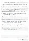
1.1.1. (b) Reduce the system to 6 u + v = 5, — 5 v = 5
; then use Back Substitution to solve
for u = 1, v = —1. 2 2
⋆
(c) Reduce the system to p + q — r = 0, —3 q + 5 r = 3, — r = 6; then solve for
p = 5, q = —11, r = —6.
(d) Reduce the system to 2 u — v + 2 w = 2, — 32 v + 4 w = 2, — w = 0; then solve for
u = 1 , v = — 4 , w = 0.
3 3
⋆ (e) Reduce the system to 5 x1 + 3 x2 — x3 = 9, 1 x2 — 2 x3 = 2 , 2 x3 = —2; then solve for
5 5 5
x1 = 4, x2 = —4, x3 = —1.
(f ) Reduce the system to x + z — 2 w = — 3, — y + 3 w = 1, — 4 z — 16w = — 4, 6w = 6; then
solve for x = 2, y = 2, z = —3, w = 1.
⋆ 1.1.2. Plugging in the values of x, y and z gives a + 2 b — c = 3, a — 2 — c = 1, 1 + 2 b + c = 2.
Solving this system yields a = 4, b = 0, and c = 1.
♥ 1.1.3. (a) With Forward Substitution, we just start with the top equation and work down.
Thus 2 x = —6 so x = —3. Plugging this into the second equation gives 12 + 3y = 3, and so
y = —3. Plugging the values of x and y in the third equation yields —3 + 4(—3) — z = 7, and
so z = —22.
⋆ (c) Start with the last equation and, assuming the coefficient of the last variable is /= 0, use
the operation to eliminate the last variable in all the preceding equations. Then, again as-
suming the coefficient of the next-to-last variable is non-zero, eliminate it from all but the
last two equations, and so on.
⋆ (d) For the systems in Exercise 1.1.1, the method works in all cases except (c) and (f ). Solv-
ing the reduced system by Forward Substitution reproduces the same solution (as it must):
(a) The system reduces to 3 x = 17 , x + 2 y = 3. (b) The reduced system is 15 u = 15 ,
2 2 2 2
3 u — 2 v = 5. (d) Reduce the system to2 3 u = 21 , 72u — v = 52, 3 u — 2 w = —1. (f ) Doesn’t
work since, after the first reduction, z doesn’t occur in the next to last equation.
√ ,
0
1.2.1. (a) 3 × 4, (b) 7, (c) 6, (d) ( —2 0 1 2 ), (e) . 2 ..
,
—6
√ , √ ,
√
.1 2 3
. 1 2 3
! 1 2 3 4, 1
. .
1.2.2. Examples: (a) .4 5 6.
,, ⋆ (b) 1 4 5
, (c) .4 5 6 7 .,, (e) . 2 ,..
7 8 9 7 8 9 3 3
! ! !
6 1 u 5
1.2.4. (b) A = , x= , b= ;
3 —2 v 5
1 ⃝c 2019 Peter J. Olver and Chehrzad Shakiban
, Chapter 1: Instructors’ Solutions Manual 3
√
, √ , √ ,
⋆ .
1 1 —1 p 0
(c) A = . 2 —1 3,
.
. , x = . q. , b = . 3. ;
, ,
—1 —1 0 r 6
√ , √ , √ ,
2 —1 2 u 2
—1 —1
.. .
. .
(d) A = 3,, x= v , , b = 1.
. .
,;
√ 3 0 ,—2 w 1
5 3 —1 √ , √ ,
x1 9
⋆
(e) A = ..
3 2 —1 . .
,, x=
. x . , b=.
2 , 5 .,;
1 1 2 x3 —1
√1 0 1 —2 , √ ,
x
√
—3 ,
. 2 —1 2 —1. . y. . —5.
(f ) A = . ., x =
. , b= . . .
.
0 —6 —4 2.
,
.
z, 2,
1 3 2 —1 w 1
1.2.5. (b) u + w = —1, u + v = —1, v + w = 2. The solution is u = —2, v = 1, w = 1.
(c) 3 x1 — x3 = 1, —2 x1 — x2 = 0, x1 + x2 — 3 x3 = 1.
The solution is x1 = 15, x2 = — 25, x3 = — 25.
⋆
(d) x + y — z — w = 0, —x + z + 2 w = 4, x — y + z = 1, 2 y — z + w = 5.
The solution is x = 2, y = 1, z = 0, w = 3.
√ , √
1 0 0 0 0 0 0 0 0 0,
. . .
0 1 0 0 0 0 0 0 0 0.
1.2.6. (a) I = . 0 0 1 0 0 ., O= 0 0 0 0 0 ..
. . .
. .
.
0 0 0 1 0, 0 0 0 0 0,
0 0 0 0 1 0 0 0 0 0
(b) I + O = I , I O = O I = O. No, it does not.
3 6 0!
1.2.7. (b) undefined, (c) , ⋆ (e) undefined,
—1 4 2√ ,
√
1 11 9, 9 —2 14
.
(f )
.
.3
.
—12 —12 .
,,
⋆ (h) . —8 6 —17 .
,.
.
7 8 8 12 —3 28
1.2.9. 1, 6, 11, 16.
√ , √2 0 0 0,
1 0 0
⋆ (b)
.
0 —2 0 0.
1.2.10. (a) 0 0 0 ., , . ..
0 0 3 0,
.
0 0 —1
0 0 0 —3
1.2.11. (a) True, ⋆ (b) true.
! !
x ! ax by ay
⋆ ♥ 1.2.12. (a) Let A = y
. Then AD = = ax = DA, so if a /= b these
z w az bw bz bw
!
a 0
are equal if and only if y = z = 0. (b) Every 2 × 2 matrix commutes with 0 a = a I.
⃝ c 2019 Peter J. Olver and Chehrzad Shakiban
All Chapters Included
for
Applied Linear
Algebra
by
Peter J. Olver
and Chehrzad Shakiban
Second Edition
Undergraduate Texts in
Mathematics
,Table of Contents
Chapter 1. Linear Algebraic Systems ................................................... 1
Chapter 2. Vector Spaces and Bases ..................................................... 22
Chapter 3. Inner Products and Norms ................................................. 40
Chapter 4. Orthogonality ........................................................................ 59
Chapter 5. Minimization and Least Squares ..................................... 77
Chapter 6. Equilibrium ......................................................................... 94
Chapter 7. Linearity ............................................................................ 105
Chapter 8. Eigenvalues and Singular Values ................................... 124
Chapter 9. Iteration .............................................................................150
Chapter 10. Dynamics ........................................................................... 176
, Instructors’ Solutions Manual for
Chapter 1: Linear Algebraic Systems
Note: Solutions marked with a ⋆ do not appear in the Students’ Solutions Manual.
1.1.1. (b) Reduce the system to 6 u + v = 5, — 5 v = 5
; then use Back Substitution to solve
for u = 1, v = —1. 2 2
⋆
(c) Reduce the system to p + q — r = 0, —3 q + 5 r = 3, — r = 6; then solve for
p = 5, q = —11, r = —6.
(d) Reduce the system to 2 u — v + 2 w = 2, — 32 v + 4 w = 2, — w = 0; then solve for
u = 1 , v = — 4 , w = 0.
3 3
⋆ (e) Reduce the system to 5 x1 + 3 x2 — x3 = 9, 1 x2 — 2 x3 = 2 , 2 x3 = —2; then solve for
5 5 5
x1 = 4, x2 = —4, x3 = —1.
(f ) Reduce the system to x + z — 2 w = — 3, — y + 3 w = 1, — 4 z — 16w = — 4, 6w = 6; then
solve for x = 2, y = 2, z = —3, w = 1.
⋆ 1.1.2. Plugging in the values of x, y and z gives a + 2 b — c = 3, a — 2 — c = 1, 1 + 2 b + c = 2.
Solving this system yields a = 4, b = 0, and c = 1.
♥ 1.1.3. (a) With Forward Substitution, we just start with the top equation and work down.
Thus 2 x = —6 so x = —3. Plugging this into the second equation gives 12 + 3y = 3, and so
y = —3. Plugging the values of x and y in the third equation yields —3 + 4(—3) — z = 7, and
so z = —22.
⋆ (c) Start with the last equation and, assuming the coefficient of the last variable is /= 0, use
the operation to eliminate the last variable in all the preceding equations. Then, again as-
suming the coefficient of the next-to-last variable is non-zero, eliminate it from all but the
last two equations, and so on.
⋆ (d) For the systems in Exercise 1.1.1, the method works in all cases except (c) and (f ). Solv-
ing the reduced system by Forward Substitution reproduces the same solution (as it must):
(a) The system reduces to 3 x = 17 , x + 2 y = 3. (b) The reduced system is 15 u = 15 ,
2 2 2 2
3 u — 2 v = 5. (d) Reduce the system to2 3 u = 21 , 72u — v = 52, 3 u — 2 w = —1. (f ) Doesn’t
work since, after the first reduction, z doesn’t occur in the next to last equation.
√ ,
0
1.2.1. (a) 3 × 4, (b) 7, (c) 6, (d) ( —2 0 1 2 ), (e) . 2 ..
,
—6
√ , √ ,
√
.1 2 3
. 1 2 3
! 1 2 3 4, 1
. .
1.2.2. Examples: (a) .4 5 6.
,, ⋆ (b) 1 4 5
, (c) .4 5 6 7 .,, (e) . 2 ,..
7 8 9 7 8 9 3 3
! ! !
6 1 u 5
1.2.4. (b) A = , x= , b= ;
3 —2 v 5
1 ⃝c 2019 Peter J. Olver and Chehrzad Shakiban
, Chapter 1: Instructors’ Solutions Manual 3
√
, √ , √ ,
⋆ .
1 1 —1 p 0
(c) A = . 2 —1 3,
.
. , x = . q. , b = . 3. ;
, ,
—1 —1 0 r 6
√ , √ , √ ,
2 —1 2 u 2
—1 —1
.. .
. .
(d) A = 3,, x= v , , b = 1.
. .
,;
√ 3 0 ,—2 w 1
5 3 —1 √ , √ ,
x1 9
⋆
(e) A = ..
3 2 —1 . .
,, x=
. x . , b=.
2 , 5 .,;
1 1 2 x3 —1
√1 0 1 —2 , √ ,
x
√
—3 ,
. 2 —1 2 —1. . y. . —5.
(f ) A = . ., x =
. , b= . . .
.
0 —6 —4 2.
,
.
z, 2,
1 3 2 —1 w 1
1.2.5. (b) u + w = —1, u + v = —1, v + w = 2. The solution is u = —2, v = 1, w = 1.
(c) 3 x1 — x3 = 1, —2 x1 — x2 = 0, x1 + x2 — 3 x3 = 1.
The solution is x1 = 15, x2 = — 25, x3 = — 25.
⋆
(d) x + y — z — w = 0, —x + z + 2 w = 4, x — y + z = 1, 2 y — z + w = 5.
The solution is x = 2, y = 1, z = 0, w = 3.
√ , √
1 0 0 0 0 0 0 0 0 0,
. . .
0 1 0 0 0 0 0 0 0 0.
1.2.6. (a) I = . 0 0 1 0 0 ., O= 0 0 0 0 0 ..
. . .
. .
.
0 0 0 1 0, 0 0 0 0 0,
0 0 0 0 1 0 0 0 0 0
(b) I + O = I , I O = O I = O. No, it does not.
3 6 0!
1.2.7. (b) undefined, (c) , ⋆ (e) undefined,
—1 4 2√ ,
√
1 11 9, 9 —2 14
.
(f )
.
.3
.
—12 —12 .
,,
⋆ (h) . —8 6 —17 .
,.
.
7 8 8 12 —3 28
1.2.9. 1, 6, 11, 16.
√ , √2 0 0 0,
1 0 0
⋆ (b)
.
0 —2 0 0.
1.2.10. (a) 0 0 0 ., , . ..
0 0 3 0,
.
0 0 —1
0 0 0 —3
1.2.11. (a) True, ⋆ (b) true.
! !
x ! ax by ay
⋆ ♥ 1.2.12. (a) Let A = y
. Then AD = = ax = DA, so if a /= b these
z w az bw bz bw
!
a 0
are equal if and only if y = z = 0. (b) Every 2 × 2 matrix commutes with 0 a = a I.
⃝ c 2019 Peter J. Olver and Chehrzad Shakiban