EC2A3 - Microeconomics II
Final Grade: 82
Notes Outline
Framework I Edgeworth Box and UPF • Week 1 - Introduction Roth (2017)
• Week 2 - General Backhouse et al. (2020)
Competitive Equilibrium
• Week 3 - Social Welfare
• Week 4 - Inequality
Framework 2 U Continuum • Week 5 - Behavioural Grubb (2015)
Economics
• Week 8 - Adverse Selection
Framework 3 State Contingent Income • Week 6 - Risk Stezka and Winter (2021)
Space • Week 7 - Insurance Market Schemiser et al. (2014)
Framework 4 State Contingent x Week 9 - Moral Hazard Lazear (2018)
Edgeworth Box
Other Lorenz Curve Model Week 4 - Inequality Starmans et al. (2017)
Frameworks Hufe et al. (2018)
Signalling Model Week 8 -Adverse Selection Wyness et al. (2021)
Public Good Games Week 10 - Public Goods and Chan et al. (2018)
Externalities Altundas et al. (2021)
Discussion Readings Summaries
Framework 1: Edgeworth Box and UPF (W1, 2, 3 & 4)
Introduction: Market System
Market System: system for producing and allocating goods and services using price signals, with 2 major
features:
(1) Decentralisation: people not coordinated explicitly on production/consumption.
(2) Self-interest: people maximising their own benefit, do not intrinsically care about others.
→ Gov Intervention: enforce property rights (endowment economy) or enforce trades at agreed prices (in
practice not always the case)
,Market Goods: goods traded at set prices in a complete market, used to measure economic activity and
guide policies.
Partial vs. General Equilibrium Model
- Partial: study of how equilibrium is determined by one market in isolation.
- General: examines the interplay of supply and demand conditions across multiple markets to
determine prices for all goods (including factor prices in cases of production)
I- General Competitive Equilibrium (GCE): Edgeworth Box
Model Set Up:
Edgeworth Box: graphic representation of pure-exchange market with 2 goods
- Combines the indifference curves (i.e., combination of preferred bundles at fixed level of utility)
of 2 consumers on 2 goods.
- Depicts an endowment economy:
𝐴
- Wealth (i.e., value of endowment): p 𝑒𝑋 for 𝑚𝐴 and 𝑒𝑌 for 𝑚𝐵 with numeraire
- Trade cannot happen outside of the box
Pareto Efficiency: allocation of goods where no one can become better off without someone else being
made worse off.
→ For well-behaved preferences, PE where allocations are tangent: 𝑀𝑅𝑆𝐴 = 𝑀𝑅𝑆𝐵
𝑀𝑈𝑋 𝑝𝑋 𝑑𝑈 𝑑𝑈
Reminder: MRS = 𝑀𝑈𝑌
= 𝑝𝑌
with 𝑀𝑈𝑋 = 𝑑𝑋
and 𝑀𝑈𝑌 = 𝑑𝑌
○ To Prove not PE: (1) 𝑀𝑅𝑆𝐴 ≠ 𝑀𝑅𝑆𝐵 or (2) find Pareto Improvement
,Contract Curve: locus of Pareto Efficient allocations in an Edgeworth Box
Shape depends on preferences
- Cobb-Douglas: Diagonal of a square box
- Perfect Substitutes: Corner Solution
- Semi-Linear: Vertical/Horizontal (ICs are horizontal shifts of
each other; m increases both purchase more of the other good)
- Perfect Complements: kink of the L-shaped
- CES Preferences: Curved, depending on substitution elasticity
Semi-Linear Examples
Derivation:
After checking that initial allocation (E) is not PE (𝑀𝑅𝑆𝐴 ≠ 𝑀𝑅𝑆𝐵 )
𝑌𝐴 𝑌𝐵
1. Along the Contract Curve, 𝑀𝑅𝑆𝐴 = 𝑀𝑅𝑆𝐵 => 𝑋𝐴
= 𝑋𝐵
2. We know that total consumption should exhaust available endowment for each good:
𝑋𝐴 + 𝑋𝐵 = 𝑋 (=10) and 𝑌𝐴 + 𝑌𝐵 = Y (=10)
𝑌𝐴 𝑌−𝑌𝐴 10−𝑌
Substituting, 𝑋𝐴
= 𝑋−𝑋𝐴
( 10−𝑋𝐴 => 𝑌𝐴 = 𝑋𝐴 , diagonal of a box)
𝐴
, General Competitive Equilibrium (Walrasian):
About Walrasian GCE:
Income Distribution in GCE Determinants:
1. Endowment Distributions (i.e., Property Rights)
2. Talent Distribution (i.e., Labour Productivity)
3. Effort Distribution (i.e., Labour Supply)
4. Market Prices
- Driven by (1) endowments: keeping preferences constant, shift in relative goods supply
changes prices.
- Driven by (2) preferences: keeping endowments constant, shift in preferences increases
demand relative to supply, increasing prices.
GCE: vector of prices and a consumption bundle for each consumer such that:
(1) Consumers maximise utility given prices
(2) Markets Clear (Total Demand = Total Supply)
𝑝𝑋
Tangency IC-Price Line: 𝑝𝑌
= 𝑀𝑅𝑆𝐴 = 𝑀𝑅𝑆𝐵
(note: every tangency is PE so GCE is PE but not all PE are in GCE)
- Existence Conditions: Continuous Aggregate Demand Functions (i.e., no jumps, small changes in
p results in small changes in demand) - satisfied with either:
(1) Convex Preferences (else: mismatch S&D) (2) Many consumers so that
discontinuous demand smoothes down
Walras’ Law: if n - 1 markets are in equilibrium, so is the nth → solve for one market (either 𝑋𝐴(𝑝𝑋, 𝑝𝑌)
or 𝑌𝐴(𝑝𝑋, 𝑝𝑌)) to find equilibrium prices.
Solving Walrasian Equilibrium:
1. Set Numeraire (𝑝𝑌 = 1 and 𝑝𝑋 = p) and write down consumers’ Budget Constraint:
𝐴 𝐴 𝐴 𝐴
For A: 𝑝𝑋𝑋𝐴 + 𝑝𝑌𝑌𝐴 ≤ 𝑝𝑋 𝐸𝑋 + 𝑝𝑌 𝐸𝑌 → 𝑝𝑋𝐴 + 𝑌𝐴 ≤ p 𝐸𝑋 + 𝐸𝑌 (=30p for (30,0))
Final Grade: 82
Notes Outline
Framework I Edgeworth Box and UPF • Week 1 - Introduction Roth (2017)
• Week 2 - General Backhouse et al. (2020)
Competitive Equilibrium
• Week 3 - Social Welfare
• Week 4 - Inequality
Framework 2 U Continuum • Week 5 - Behavioural Grubb (2015)
Economics
• Week 8 - Adverse Selection
Framework 3 State Contingent Income • Week 6 - Risk Stezka and Winter (2021)
Space • Week 7 - Insurance Market Schemiser et al. (2014)
Framework 4 State Contingent x Week 9 - Moral Hazard Lazear (2018)
Edgeworth Box
Other Lorenz Curve Model Week 4 - Inequality Starmans et al. (2017)
Frameworks Hufe et al. (2018)
Signalling Model Week 8 -Adverse Selection Wyness et al. (2021)
Public Good Games Week 10 - Public Goods and Chan et al. (2018)
Externalities Altundas et al. (2021)
Discussion Readings Summaries
Framework 1: Edgeworth Box and UPF (W1, 2, 3 & 4)
Introduction: Market System
Market System: system for producing and allocating goods and services using price signals, with 2 major
features:
(1) Decentralisation: people not coordinated explicitly on production/consumption.
(2) Self-interest: people maximising their own benefit, do not intrinsically care about others.
→ Gov Intervention: enforce property rights (endowment economy) or enforce trades at agreed prices (in
practice not always the case)
,Market Goods: goods traded at set prices in a complete market, used to measure economic activity and
guide policies.
Partial vs. General Equilibrium Model
- Partial: study of how equilibrium is determined by one market in isolation.
- General: examines the interplay of supply and demand conditions across multiple markets to
determine prices for all goods (including factor prices in cases of production)
I- General Competitive Equilibrium (GCE): Edgeworth Box
Model Set Up:
Edgeworth Box: graphic representation of pure-exchange market with 2 goods
- Combines the indifference curves (i.e., combination of preferred bundles at fixed level of utility)
of 2 consumers on 2 goods.
- Depicts an endowment economy:
𝐴
- Wealth (i.e., value of endowment): p 𝑒𝑋 for 𝑚𝐴 and 𝑒𝑌 for 𝑚𝐵 with numeraire
- Trade cannot happen outside of the box
Pareto Efficiency: allocation of goods where no one can become better off without someone else being
made worse off.
→ For well-behaved preferences, PE where allocations are tangent: 𝑀𝑅𝑆𝐴 = 𝑀𝑅𝑆𝐵
𝑀𝑈𝑋 𝑝𝑋 𝑑𝑈 𝑑𝑈
Reminder: MRS = 𝑀𝑈𝑌
= 𝑝𝑌
with 𝑀𝑈𝑋 = 𝑑𝑋
and 𝑀𝑈𝑌 = 𝑑𝑌
○ To Prove not PE: (1) 𝑀𝑅𝑆𝐴 ≠ 𝑀𝑅𝑆𝐵 or (2) find Pareto Improvement
,Contract Curve: locus of Pareto Efficient allocations in an Edgeworth Box
Shape depends on preferences
- Cobb-Douglas: Diagonal of a square box
- Perfect Substitutes: Corner Solution
- Semi-Linear: Vertical/Horizontal (ICs are horizontal shifts of
each other; m increases both purchase more of the other good)
- Perfect Complements: kink of the L-shaped
- CES Preferences: Curved, depending on substitution elasticity
Semi-Linear Examples
Derivation:
After checking that initial allocation (E) is not PE (𝑀𝑅𝑆𝐴 ≠ 𝑀𝑅𝑆𝐵 )
𝑌𝐴 𝑌𝐵
1. Along the Contract Curve, 𝑀𝑅𝑆𝐴 = 𝑀𝑅𝑆𝐵 => 𝑋𝐴
= 𝑋𝐵
2. We know that total consumption should exhaust available endowment for each good:
𝑋𝐴 + 𝑋𝐵 = 𝑋 (=10) and 𝑌𝐴 + 𝑌𝐵 = Y (=10)
𝑌𝐴 𝑌−𝑌𝐴 10−𝑌
Substituting, 𝑋𝐴
= 𝑋−𝑋𝐴
( 10−𝑋𝐴 => 𝑌𝐴 = 𝑋𝐴 , diagonal of a box)
𝐴
, General Competitive Equilibrium (Walrasian):
About Walrasian GCE:
Income Distribution in GCE Determinants:
1. Endowment Distributions (i.e., Property Rights)
2. Talent Distribution (i.e., Labour Productivity)
3. Effort Distribution (i.e., Labour Supply)
4. Market Prices
- Driven by (1) endowments: keeping preferences constant, shift in relative goods supply
changes prices.
- Driven by (2) preferences: keeping endowments constant, shift in preferences increases
demand relative to supply, increasing prices.
GCE: vector of prices and a consumption bundle for each consumer such that:
(1) Consumers maximise utility given prices
(2) Markets Clear (Total Demand = Total Supply)
𝑝𝑋
Tangency IC-Price Line: 𝑝𝑌
= 𝑀𝑅𝑆𝐴 = 𝑀𝑅𝑆𝐵
(note: every tangency is PE so GCE is PE but not all PE are in GCE)
- Existence Conditions: Continuous Aggregate Demand Functions (i.e., no jumps, small changes in
p results in small changes in demand) - satisfied with either:
(1) Convex Preferences (else: mismatch S&D) (2) Many consumers so that
discontinuous demand smoothes down
Walras’ Law: if n - 1 markets are in equilibrium, so is the nth → solve for one market (either 𝑋𝐴(𝑝𝑋, 𝑝𝑌)
or 𝑌𝐴(𝑝𝑋, 𝑝𝑌)) to find equilibrium prices.
Solving Walrasian Equilibrium:
1. Set Numeraire (𝑝𝑌 = 1 and 𝑝𝑋 = p) and write down consumers’ Budget Constraint:
𝐴 𝐴 𝐴 𝐴
For A: 𝑝𝑋𝑋𝐴 + 𝑝𝑌𝑌𝐴 ≤ 𝑝𝑋 𝐸𝑋 + 𝑝𝑌 𝐸𝑌 → 𝑝𝑋𝐴 + 𝑌𝐴 ≤ p 𝐸𝑋 + 𝐸𝑌 (=30p for (30,0))